The Complete Guide to Time Series Forecasting using Sklearn, Pandas and Numpy

There are many so-called traditional models for time series forecasting, such as the SARIMAX family of models, exponential smoothing, or BATS and TBATS.

However, very few times do we mention the most common machine learning models for regression, such as decision trees, random forests, gradient boosting, or even a support vector regressor. We see these models applied extensively in typical regression problems, but not for time series forecasting.

Hence the reason of writing this article! Here, we design a framework to frame a time series problem as a supervised learning problem, allowing us to use any model we want from our favourite library: scikit-learn!

By the end of this article, you will have the tools and knowledge to apply any machine learning model for time series forecasting along with the statistical models mentioned above.

Let’s get started!

The full source code is available on GitHub.

Learn the latest time series analysis techniques with my free time series cheat sheet in Python! Get the implementation of statistical and deep learning techniques, all in Python and TensorFlow!

Preparing the dataset

First, we import all the libraries required to complete our tutorial. 

import numpy as np
import pandas as pd
import statsmodels.api as sm
import matplotlib.pyplot as plt

Here, we use the statsmodels library to import the dataset, which is the weekly CO2 concentration from 1958 to 2001.

data = sm.datasets.co2.load_pandas().data

A good first step is to visualize our data with the following code block.

fig, ax = plt.subplots(figsize=(16, 11))

ax.plot(data['co2'])
ax.set_xlabel('Time')
ax.set_ylabel('CO2 concentration (ppmw)')

fig.autofmt_xdate()
plt.tight_layout()

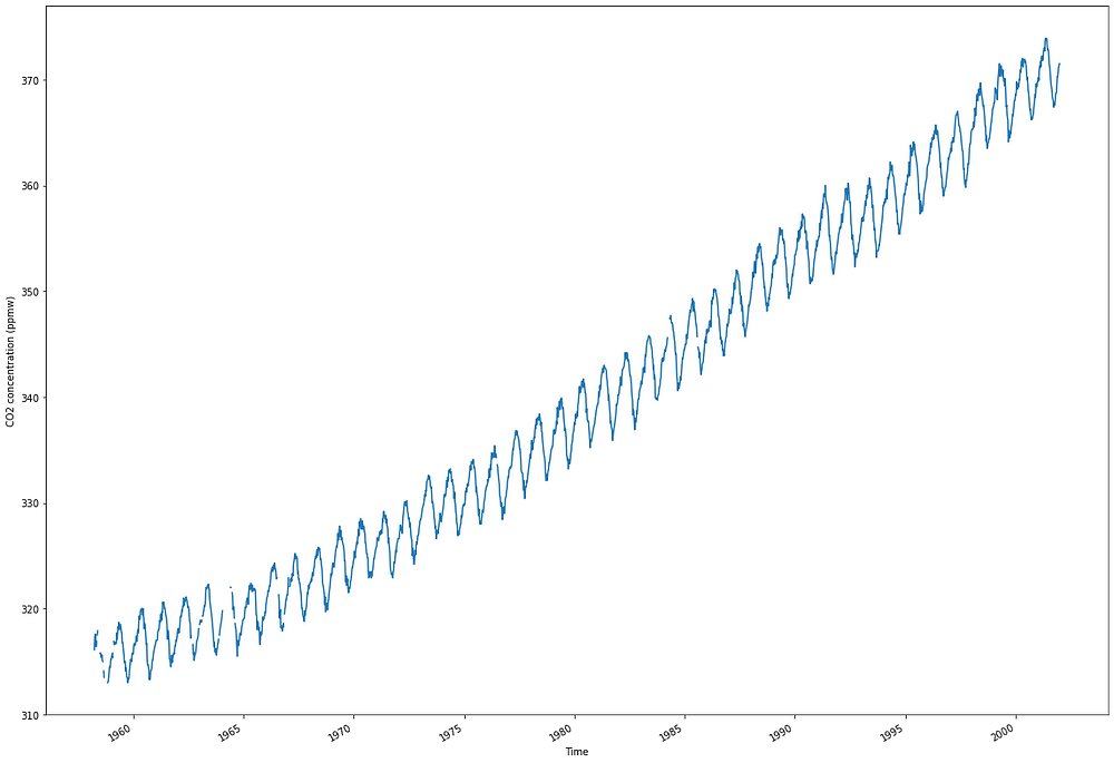
From the image above, we notice a clear positive trend in the data, as the concentration is increasing over time. We also observe a yearly seasonal pattern. This is due to the change of seasons, where CO2 concentration is higher during winter than during summer. Finally, we see some missing data at the beginning of the dataset. 

Let’s then treat that missing data using interpolation. We will simply take a linear interpolation between two known points to fill the missing values.

data = data.interpolate()

Now that we have no missing data, we are ready to get started with modeling!

Modeling with scikit-learn

As you will see, the biggest challenge in forecasting time series with scikit-learn is in setting up the problem correctly.

There are 3 different ways in which we can frame a time series forecasting problem as a supervised learning problem:

1. Predict the next time step using the previous observation
2. Predict the next time step using a sequence of past observations
3. Predict a sequence of future time steps using a sequence of past observations

Let’s explore each situation in details!

Predict the next time step using the previous observation

This is the most basic setup. The model outputs a prediction for the next time step, given only the previous observation, as shown in the figure below.

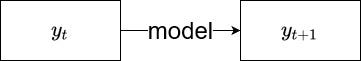
This is a simple use case with little practical applications, since a model is likely not going to learn anything from the previous observation only. However, it serves as a good starting point to help us understand the more complex scenarios later on.

So, at the moment, our dataset looks like this:

Which is not very useful. Right, all the values are in single column, but we need to format the dataset such that the current observation is a feature to predict the next observation (the target).

Thus, we add a second column that simply shifts the co2 column such that the value in 1958–03–29 is now a predictor for the value in 1958–04–05.

df = data.copy()

df['y'] = df['co2'].shift(-1)

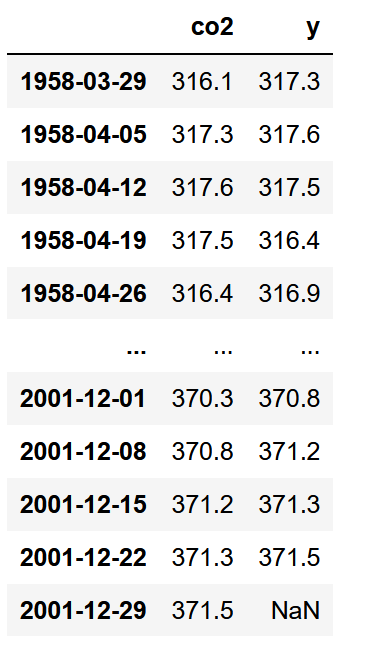
As you can, our dataset is now formatted such that each current observation is a predictor for the next observation! Notice that we have a missing value of the end of our dataset. This is normal for the last known observation. We will remove this row in a future step.

For now, let’s separate our dataset into a training and test set, in order to run our models and evaluate them. Here, we use the last two years of data for the training set. Since we have weekly data, and there are 52 weeks in a year, it means that the last 104 samples are kept for the test set.

train = df[:-104]
test = df[-104:]
test = test.drop(test.tail(1).index) # Drop last row

Baseline model

Of course, we need a baseline model to determine if using machine learning models is better. Here, we naively predict that the next observation will have the same value as the current observation.

In other words, we simply set the co2 column as our baseline predictions.

test = test.copy()
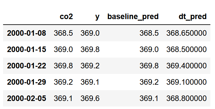
test['baseline_pred'] = test['co2']

Great! With this step done, let’s move on to more complex models.

Decision Tree

Here, let’s apply a decision tree regressor. This model can be replaced by any model you want from the scikit-learn library! Note that we use a random state to ensure reproducibility.

from sklearn.tree import DecisionTreeRegressor

X_train = train['co2'].values.reshape(-1,1)
y_train = train['y'].values.reshape(-1,1)
X_test = test['co2'].values.reshape(-1,1)

# Initialize the model
dt_reg = DecisionTreeRegressor(random_state=42)

# Fit the model
dt_reg.fit(X=X_train, y=y_train)

# Make predictions
dt_pred = dt_reg.predict(X_test)

# Assign predictions to a new column in test
test['dt_pred'] = dt_pred

Notice that we keep the modeling portion simple. We don’t perform any cross-validation or hyperparameter tuning, although those techniques can be applied here normally, just like in any other regression problem. 

Feel free to apply those techniques and see if you can get better performances.

Gradient boosting

For the sake of trying different models, let’s now apply gradient boosting.

from sklearn.ensemble import GradientBoostingRegressor

gbr = GradientBoostingRegressor(random_state=42)

gbr.fit(X_train, y=y_train.ravel())

gbr_pred = gbr.predict(X_test)

test['gbr_pred'] = gbr_pred

Great! We now have predictions from two machine learning models and a baseline. It is time to evaluate the performance of each method.

Evaluation

Here, we use the mean absolute percentage error (MAPE). It is an especially informative error metric, as it return a percentage, which is easy to interpret. Make sure to only apply it when you don’t have values close to 0, which is the case here.

Unfortunately, MAPE is not implemented yet in scikit-learn, so we must define the function by hand.

def mape(y_true, y_pred):
    return round(np.mean(np.abs((y_true - y_pred) / y_true)) * 100, 2)

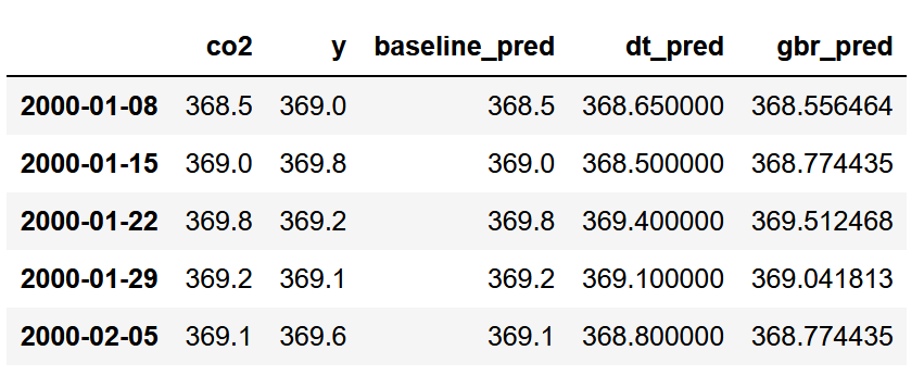
Then, we can evaluate each model and generate the following bar plot:

baseline_mape = mape(test['y'], test['baseline_pred'])
dt_mape = mape(test['y'], test['dt_pred'])
gbr_mape = mape(test['co2'], test['gbr_pred'])

# Generate bar plot
fig, ax = plt.subplots(figsize=(7, 5))

x = ['Baseline', 'Decision Tree', 'Gradient Boosting']
y = [baseline_mape, dt_mape, gbr_mape]

ax.bar(x, y, width=0.4)
ax.set_xlabel('Regressor models')
ax.set_ylabel('MAPE (%)')
ax.set_ylim(0, 0.3)

for index, value in enumerate(y):
    plt.text(x=index, y=value + 0.02, s=str(value), ha='center')
    
plt.tight_layout()

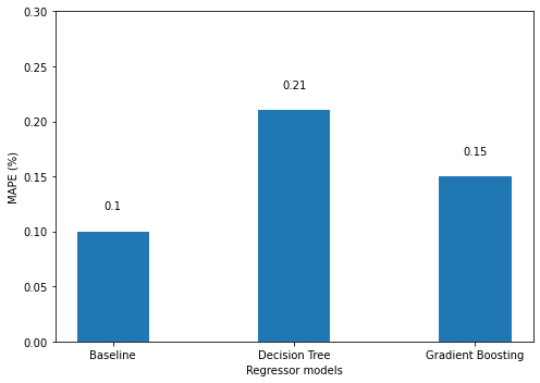
Looking at the figure above, we see that the baseline has the best performance, since it has the lowest MAPE. This makes sense as the CO2 concentration does not seem to change drastically from one week to another.

In this case, using machine learning models did not give us any added value. Again, this might be because the model is only learning from one observation to make a prediction. It might be better to give it a sequence as input, in order to predict the next time step.

This brings us to the next scenario!

Predict the next time step using a sequence of past observations

As we have seen in the previous example, using a single observation to predict the next time step did not work very well. Now, let’s try using a sequence as input to the model and predict the next time step, as shown below

Again, we must format our dataset such that we have a sequence of past observations acting as predictors to the following time step. 

We can easily write a function that adds shifted columns to get the desired input length.

def window_input(window_length: int, data: pd.DataFrame) -> pd.DataFrame:
    
    df = data.copy()
    
    i = 1
    while i < window_length:
        df[f'x_{i}'] = df['co2'].shift(-i)
        i = i + 1
        
    if i == window_length:
        df['y'] = df['co2'].shift(-i)
        
    # Drop rows where there is a NaN
    df = df.dropna(axis=0)
        
    return df

Let’s use this function to have an input of 5 observations in order to predict the next time step.

new_df = window_input(5, data)

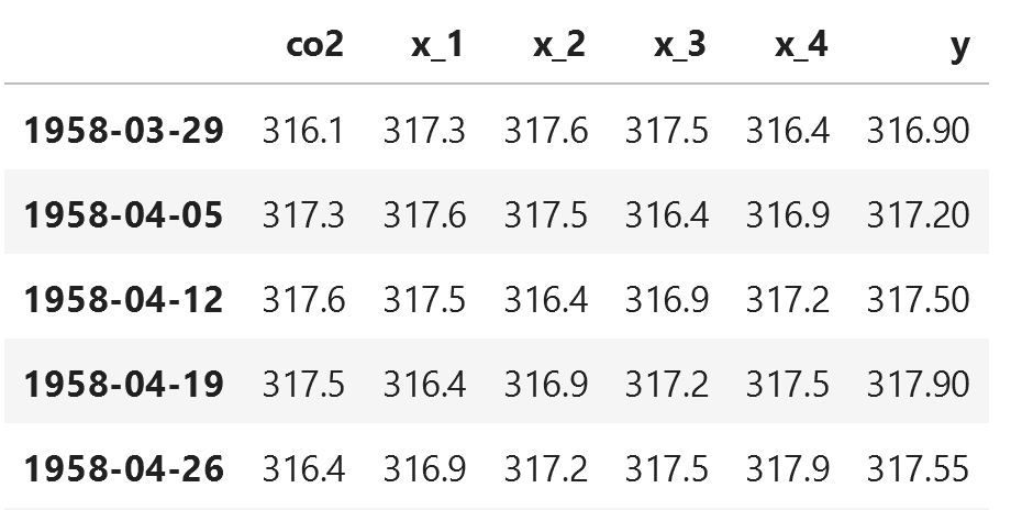
Looking at the figure above, we can see that our dataset is arranged in such a way that we have five observations to predict the next time step, stored in the y column.

This essentially takes care of the hardest part! Now, it is simply matter of applying different models and seeing which performs best.

Before heading to that step, let’s first split our data into a training and a test set.

from sklearn.model_selection import train_test_split

X = new_df[['co2', 'x_1', 'x_2', 'x_3', 'x_4']].values
y = new_df['y'].values

X_train, X_test, y_train, y_test = train_test_split(X, y, test_size=0.3, random_state=42, shuffle=False)

Baseline model

Again, let’s define a baseline model for this situation. Here, we will simply predict the mean of the input sequence

baseline_pred = []

for row in X_test:
    baseline_pred.append(np.mean(row))

Decision tree

Again, let’s apply a decision tree regressor. This is as simple as the previous implementation.

dt_reg_5 = DecisionTreeRegressor(random_state=42)

dt_reg_5.fit(X_train, y_train)

dt_reg_5_pred = dt_reg_5.predict(X_test)

Gradient boosting

For the sake of consistency, let’s also try gradient boosting.

gbr_5 = GradientBoostingRegressor(random_state=42)

gbr_5.fit(X_train, y_train.ravel())

gbr_5_pred = gbr_5.predict(X_test)

Evaluation

We can now evaluate the performance of each model. Again, we use the MAPE and plot the results in a bar plot. This is essentially the same code as before.

baseline_mape = mape(y_test, baseline_pred)
dt_5_mape = mape(y_test, dt_reg_5_pred)
gbr_5_mape = mape(y_test, gbr_5_pred)

# Generate the bar plot

fig, ax = plt.subplots()

x = ['Baseline', 'Decision Tree', 'Gradient Boosting']
y = [baseline_mape, dt_5_mape, gbr_5_mape]

ax.bar(x, y, width=0.4)
ax.set_xlabel('Regressor models')
ax.set_ylabel('MAPE (%)')
ax.set_ylim(0, 2.5)

for index, value in enumerate(y):
    plt.text(x=index, y=value + 0.1, s=str(value), ha='center')
    
plt.tight_layout()

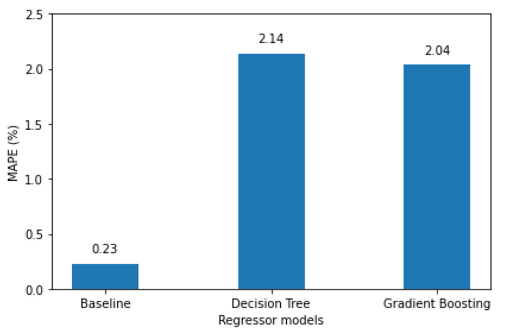
Surprisingly, from the figure above, we see that the machine learning models do not outperform the baseline. 

While hyperparameter tuning can likely increase the performance of the ML models, I suspect that suspect that input window is too short. An input of five weeks is not enough for the model to pick up the trend and seasonal components, so we might need a longer window of time.

We will try exactly that in the next scenario!

Predict a sequence of future time steps using a sequence of past observations

The final scenario is using a sequence of observations to predict a sequence of future time steps, as shown below.

Here, our model is required to output a sequence of predictions. This can be seen as a multi-output regression problem.

So, the first step is to format our dataset appropriately. We develop another function that uses the shift method to format the dataset as a multi-output regression problem.

def window_input_output(input_length: int, output_length: int, data: pd.DataFrame) -> pd.DataFrame:
    
    df = data.copy()
    
    i = 1
    while i < input_length:
        df[f'x_{i}'] = df['co2'].shift(-i)
        i = i + 1
        
    j = 0
    while j < output_length:
        df[f'y_{j}'] = df['co2'].shift(-output_length-j)
        j = j + 1
        
    df = df.dropna(axis=0)
    
    return df

Here, we will use a sequence of 26 observations to predict the next 26 time steps. In other words, we input half of a year to predict the next half. Note that the input and output sequences do not need to have the same length. This is an arbitrary decision on my end.

seq_df = window_input_output(26, 26, data)

As you can see, we now have a dataset where 26 observations are used as predictors for the next 26 time steps.

Before moving on to modeling, again, we will split the data into a training and a test set. Here, we reserve the last two rows for the test set, as it gives us 52 test samples.

X_cols = [col for col in seq_df.columns if col.startswith('x')]

X_cols.insert(0, 'co2')

y_cols = [col for col in seq_df.columns if col.startswith('y')]

X_train = seq_df[X_cols][:-2].values
y_train = seq_df[y_cols][:-2].values

X_test = seq_df[X_cols][-2:].values
y_test = seq_df[y_cols][-2:].values

Baseline model

As a baseline model, we will simply repeat the input sequence. In other words, we take the input sequence and output the same sequence as our baseline predictions.

This is a very trivial prediction, so we’ll implement it when we are ready to evaluate the models.

Decision tree

Again, let’s try applying a decision tree. Note that a decision tree can produce multi-output predictions, so we don’t need to do any extra work here.

dt_seq = DecisionTreeRegressor(random_state=42)

dt_seq.fit(X_train, y_train)

dt_seq_preds = dt_seq.predict(X_test)

Gradient boosting

Now, gradient boosting takes a bit of extra work. It cannot handle a multi-output target. Trying to fit a gradient boosting model immediately will result in an error.

Here, we must wrap the model such that its prediction is used as an input to feed the next prediction. This is achieved using the RegressorChain wrapper from scikit-learn.

from sklearn.multioutput import RegressorChain

gbr_seq = GradientBoostingRegressor(random_state=42)

chained_gbr = RegressorChain(gbr_seq)

chained_gbr.fit(X_train, y_train)

gbr_seq_preds = chained_gbr.predict(X_test)

This allowed to train the model and make predictions without encountering any errors. As I mentioned, behind the scenes, the model predicts the next time step, and uses that prediction to make the next prediction. The drawback of that method is that if the first prediction is bad, then the rest of the sequence is likely going to be bad.

Let’s evaluate each model now.

Evaluation

Again, we use the MAPE to evaluate our forecasting methods.

mape_dt_seq = mape(dt_seq_preds.reshape(1, -1), y_test.reshape(1, -1))
mape_gbr_seq = mape(gbr_seq_preds.reshape(1, -1), y_test.reshape(1, -1))
mape_baseline = mape(X_test.reshape(1, -1), y_test.reshape(1, -1))

# Generate the bar plot

fig, ax = plt.subplots()

x = ['Baseline', 'Decision Tree', 'Gradient Boosting']
y = [mape_baseline, mape_dt_seq, mape_gbr_seq]

ax.bar(x, y, width=0.4)
ax.set_xlabel('Regressor models')
ax.set_ylabel('MAPE (%)')
ax.set_ylim(0, 1)

for index, value in enumerate(y):
    plt.text(x=index, y=value + 0.05, s=str(value), ha='center')
    
plt.tight_layout()

From the figure above, we can see that we finally managed to train ML models that outperform the baseline! Here, the decision tree model is the champion model, as it achieves the lowest MAPE.

We optionally visualize the predictions over the last year.

fig, ax = plt.subplots(figsize=(16, 11))ax.plot(np.arange(0, 26, 1), X_test[1], 'b-', label='input')
ax.plot(np.arange(26, 52, 1), y_test[1], marker='.', color='blue', label='Actual')
ax.plot(np.arange(26, 52, 1), X_test[1], marker='o', color='red', label='Baseline')
ax.plot(np.arange(26, 52, 1), dt_seq_preds[1], marker='^', color='green', label='Decision Tree')
ax.plot(np.arange(26, 52, 1), gbr_seq_preds[1], marker='P', color='black', label='Gradient Boosting')ax.set_xlabel('Timesteps')
ax.set_ylabel('CO2 concentration (ppmv)')plt.xticks(np.arange(1, 104, 52), np.arange(2000, 2002, 1))
plt.legend(loc=2)fig.autofmt_xdate()
plt.tight_layout()

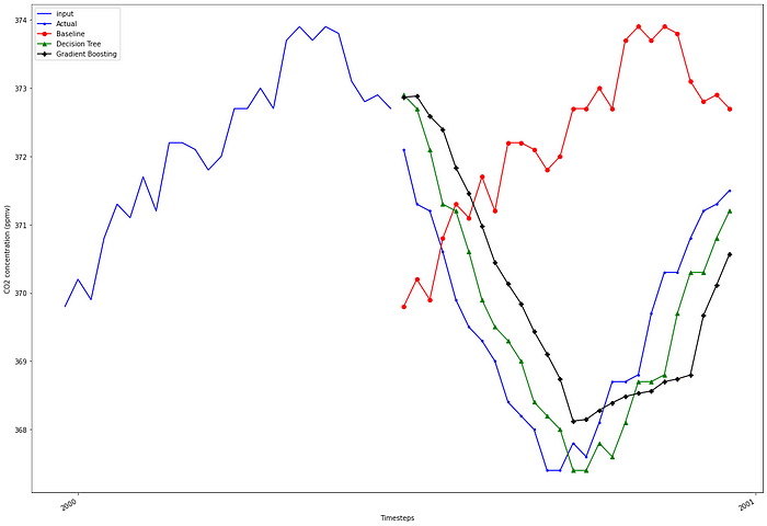
Further supporting the MAPE, we can see that the decision tree and gradient boosting follow the actual values more closely than the baseline predictions.

In this article, we saw how to frame a time series forecasting problem as a regression problem that can be solved using scikit-learn regression models.

We explored the following scenarios:

1. Predict the next time step using the previous observation
2. Predict the next time step using a sequence of past observations
3. Predict a sequence of future time steps using a sequence of past observations

We now have a framework to frame any time series forecasting problem as a supervised learning problem, where you can apply any regressor model from scikit-learn.

I hope you found this article useful!

Make sure to download my free time series forecasting cheat sheet in Python, covering both statistical and deep learning models!

Cheers! 🍺

Support me

Enjoying my work? Show your support with Buy me a coffee, a simple way for you to encourage me, and I get to enjoy a cup of coffee! If you feel like it, just click the button below 👇