All About N-HiTS: The Latest Breakthrough in Time Series Forecasting

In a previous article, we explored N-BEATS: a deep learning model relying on the concept of basis expansion to forecast time series. 

At the time of the release,in 2020, N-BEATS achieved state-of-the-art results using a pure deep learning architecture that did not rely on time-series-specific components.

As of January 2022, a new model that enhances N-BEATS has been proposed: N-HiTS. This new model proposed by Challu and Olivares et al. improves the treatment of the input, and the construction of the output, resulting in better accuracy and lower computational costs.

In this article, we first explore in details the inner workings of N-HiTS to understand how this new method improves upon N-BEATS. Then, we use Python to actually apply N-HiTS in a forecasting project.

I strongly recommend that you read my article on N-BEATS before tackling this one, as N-HiTS is an evolution of N-BEATS, and many concepts are shared between both models.

Again, I will use more intuition and less equations to explain the architecture of N-HiTS. Of course, for more details, I suggest that you read the original paper.

Learn the latest time series analysis techniques with my free time series cheat sheet in Python! Get the implementation of statistical and deep learning techniques, all in Python and TensorFlow!

Let’s get started!

Exploring N-HiTS

N-HiTS stands for Neural Hierarchical interpolation for Time Series forecasting.

In short, N-HiTS is an extension of the N-BEATS model that improves the accuracy of the predictions and reduces the computational cost. This is achieved by the model sampling the time series at different rates. That way, the model can learn short-term and long-term effects in the series. Then, when generating the predictions, it will combine the forecasts made at different time scales, considering both long-term and short-term effects. This is called hierarchical interpolation.

Let’s dive deeper into the architecture to see, in details, how the model works.

The architecture of N-HiTS

Below is the architecture of N-HiTS.

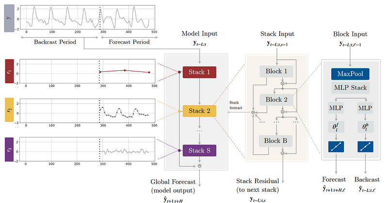
From the picture above, we notice that the model is very similar to N-BEATS: the model makes both a forecast and backcast, it is made of stacks and blocks, the final prediction is the sum of the partial predictions of each stack, and there are residual connections between each block in a stack.

However, there are some key modifications that allow N-HiTS to consistently outperform N-BEATS.

Multi-rate signal sampling

At the block-level, we notice the addition of a MaxPool layer. This is how the model achieves multi-rate sampling.

Recall that maxpooling simply takes the largest value in a given set of values. Each stack has its own kernel size, and the length of the kernel size determines the rate of sampling. 

A large kernel size means that the stack focuses on long-term effects in the time series. Alternatively, a small kernel size emphasizes short-term effects in the series. This is visualized in the figure below.

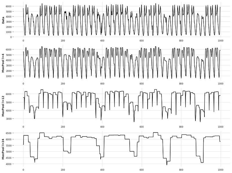
Looking at the picture above, we can see how varying the kernel size impacts the input signal of a stack. With a small kernel size, the series is almost unchanged and contains short-term variations. However, as the kernel size increases, we can see that the series is more aggressively smoothed and long-term variations are emphasized. 

Thus, it is the MaxPool layer that allows each stack to focus on a specific signal scale, either short-term or long-term. This is also what allows N-HiTS to perform better on long horizon forecasting, because there is a stack that specializes in learning and predicting long-term effects in the series.

Also, since large kernel size resamples the series more aggressively, it reduces the number of learnable parameters, thus making the model lighter and faster to train.

Regression

Once the input signal passes the MaxPool layer, the block uses fully-connected networks to perform a regression and output a forecast and a backcast. 

The backcast represents the information captured by the block. So, we remove the backcast from the input signal and pass the resulting signal to the next block through residual connections. That way, any information not captured by a certain block can be modeled by the next.

Hierarchical interpolation

As the name suggests, N-HiTS uses hierarchical interpolation to produce its predictions. This is used to reduce the cardinality of the predictions. Let’s translate this to everyday language.

Remember that the cardinality is simply the number of elements in a given set of numbers. For example, the cardinality of [6,7,8,9] is 4, since there are four elements in the set.

So, in most forecasting models, the cardinality of the predictions is equal to the length of the forecast horizon. In other words, the number of predictions equals the number of future timesteps we wish to predict. For example, if we want hourly predictions for the next 24h, then the model must output 24 predictions.

Of course, all of this makes sense, but it can become problematic when the horizon becomes very long. What if, instead of hourly predictions of the next 24h, we want hourly predictions of the next seven days. In that case, the model’s output has a cardinality of 168 (24 * 7). 

If you recall the N-BEATS model, the final predictions is the combination of all partial predictions of each stack. Therefore, each stack is generating 168 predictions, which is computationally expensive.

To combat that, N-HiTS uses hierarchical interpolation, where each stack has what they call an expressiveness ratio. This is simply the number of predictions per unit of time. In turn, this relates to the fact that each stack specializes in treating the series at a different rate, because the MaxPool layer subsamples the series. 

For example, one stack is learning short-term effects at every hour, but the next one subsamples the series at every 12h, and the next one at every 24h. Therefore, since each stack specializes in its own scale, the cardinality is different for each. This is illustrated in the figure below.

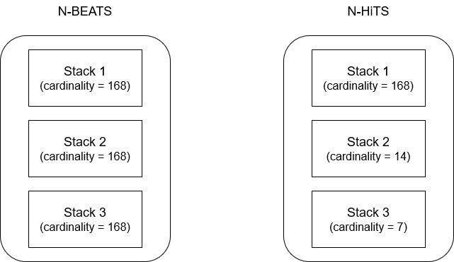
In the picture above, we assume a scenario where we have hourly data, and we wish to make hourly predictions for the next week (168 predictions into the future). In the case of N-BEATS, each stack is making 168 partial predictions and each must be summed to generate the final predictions.

However, in the case of N-HiTS, each stack looks at the data at a different scale, due to the MaxPool layer. Therefore, Stack 1 looks at the hourly data, and therefore must make 168 predictions. Stack 2, for example, looks at the data every 12h, and therefore will only have to make 14 predictions (because 12 fits 14 times in 168). Then, Stack 3 looks at the data every 24h, so it only has to make 7 predictions (because 24 fits 7 times in 168).

Thus, we see that Stack 1 has a higher expressiveness ratio than Stack 2, which has a higher expressiveness ratio than Stack 3.

We can visualize this behaviour in the figure below.

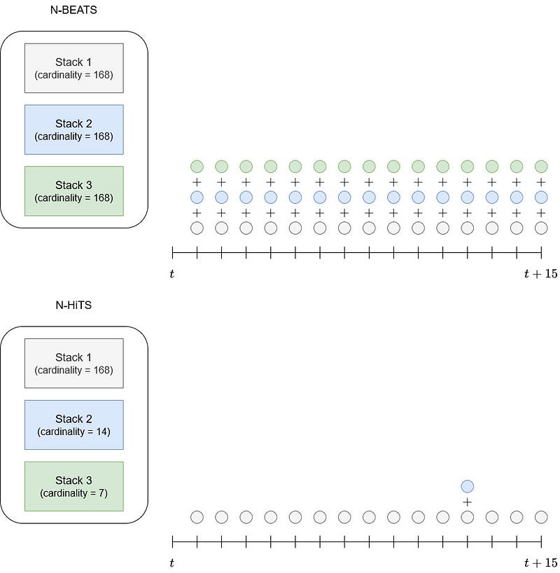
From the picture above, we clearly see that N-BEATS has each of its stack output a prediction at every timestep, and each must be summed to generate a final prediction.

On the other hand, N-HiTS has stacks that work at different frequencies. Therefore, Stack 1 is making a prediction at every timestep, but Stack 2 only makes a prediction every 12h, and Stack 3 every 24h, hence reducing the computation cost.

The fact of combining predictions at different time scales is what defines hierarchical interpolation.

If it is not clear, here is a figure taken from the original article that also illustrates hierarchical interpolation.

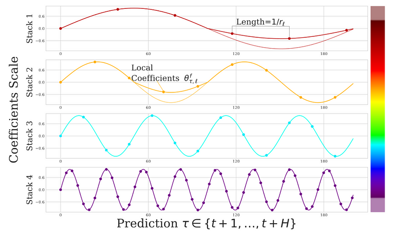
Again, in the picture above, we see that each stack in N-HiTS outputs a different number of predictions, because each stack works at a different frequency. Stack 1 looks at long-term effects, and so its predictions are more spaced in time. On the other hand, Stack 4 looks at short-term effects and outputs more granular predictions that are closer in time.

N-HiTS in summary

In short, N-HiTS extends the N-BEATS architecture with a MaxPool layer that allows each stack to look at the series at a different scale. One stack can specialize in long-term effects, and another on short-term effects. The final prediction is obtained by combining the predictions of each stack in a process called hierarchical interpolation. This makes the model lighter, and more accurate for predicting long horizons.

Now that we have explored the inner workings of N-HiTS in details, let’s apply it in a forecasting project.

Forecasting with N-HiTS

We are now ready to apply the N-HiTS model in a forecasting project. Here, we will predict the hourly Interstate 94 Westbound traffic volume. Note that we use only a sample of the full dataset available on UCI machine learning repository, kindly provided by the MN Department of Transportation.

This is the same dataset that we used in the article of N-BEATS. We will use the same baseline and the same train/test split, to evaluate the performance of N-HiTS against N-BEATS and the baseline model. 

For completeness, we include all the steps here, but if you recently read my article on N-BEATS, feel free to jump straight to applying N-HiTS.

Again, we use Darts, all the code is in Python and you can grab the full source code, as well as the dataset, on GitHub.

Let’s go!

Read the data

Of course, every project starts off with importing the necessary libraries.

import pandas as pd
import numpy as np
import datetime
import matplotlib.pyplot as plt

from darts import TimeSeries

import warnings
warnings.filterwarnings('ignore')

Then, we actually read our data and store it in a DataFrame.

df = pd.read_csv('data/daily_traffic.csv')

Since we are working with Darts, we will go from DataFrame to a TimeSeries object, which is the fundamental object in Darts. Every model in Darts must have a TimeSeries object as input, and it outputs a TimeSeries object as well.

series = TimeSeries.from_dataframe(df, time_col='date_time')

Now, we can easily visualize our data using the plot method.

series.plot()

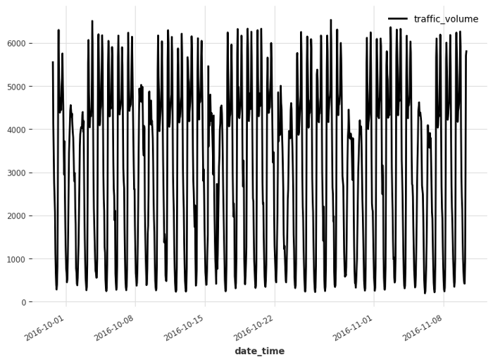
Looking at the figure above, we already identify that we have two seasonal periods: weekly and daily. Clearly, there are more cars on the road during the day than at night, and there are more cars during the week than on the weekend.

This can actually be verified using Darts. It comes with a check_seasonality function that can tell us if a seasonal period has statistical significance.

In this case, since we have hourly data, a daily seasonality has a period of 24 (24 hours in a day), and a weekly seasonality has a period of 168 (24*7 hours in a week).

So, let’s make sure that both seasonal periods are significant.

from darts.utils.statistics import check_seasonality

is_daily_seasonal, daily_period = check_seasonality(series, m=24, max_lag=400, alpha=0.05)
is_weekly_seasonal, weekly_period = check_seasonality(series, m=168, max_lag=400, alpha=0.05)

print(f'Daily seasonality: {is_daily_seasonal} - period = {daily_period}')
print(f'Weekly seasonality: {is_weekly_seasonal} - period = {weekly_period}')

The code block above will print that both seasonal periods are significant, and we will later how we can encode that information to feed it to our model.

Split the data

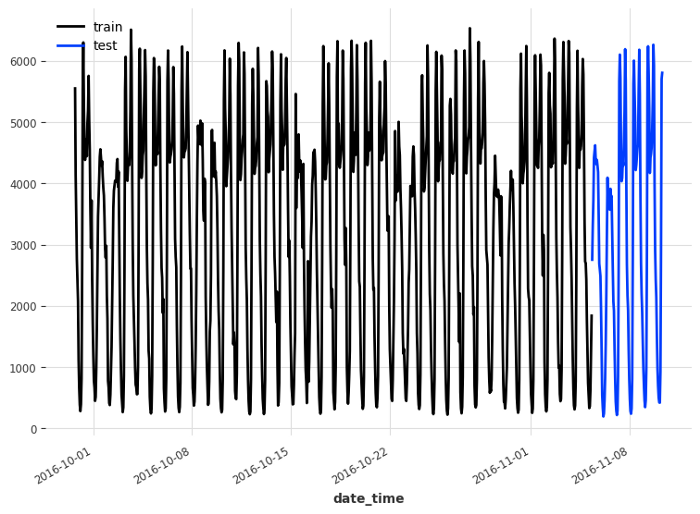
A natural step in a forecasting project to split our data into a training and test set. In this case, we reserve the last five days of data for the test set, and use the rest for training.

train, test = series[:-120], series[-120:]

train.plot(label='train')
test.plot(label='test')

Baseline model

Before using N-BEATS it is good to have a baseline model first. This is a simple model that serves as a benchmark to determine if a more complex model is actually better.

A baseline model usually relies on simple statistics or a simple heuristic. In this case, a naive forecasting method can be to simply repeat the last season. Here, since we have two seasonal periods, we will use the weekly seasonality, to consider that traffic volume is lower on the weekends.

from darts.models.forecasting.baselines import NaiveSeasonal

naive_seasonal = NaiveSeasonal(K=168)
naive_seasonal.fit(train)

pred_naive = naive_seasonal.predict(120)

In the code block above, we simply take the last week of data in the training set and repeat it into the future. Of course, since our forecast horizon has only five days instead of seven, we truncate the predictions at the fifth day.

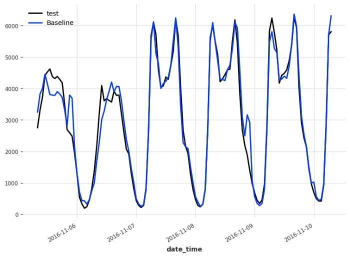
Below, we can visualize the forecasts coming from the baseline model.

test.plot(label='test')
pred_naive.plot(label='Baseline')

Then, we evaluate the performance of the baseline using the mean absolute error (MAE).

from darts.metrics import mae

naive_mae = mae(test, pred_naive)

print(naive_mae)

This gives us a MAE of 249, and it is thus the score that we try to beat using N-HiTS.

Applying N-HiTS

We are now ready to apply N-HiTS to our project.

Darts makes it very easy for us to use state-of-the-art models like N-BEATS and N-Hits, so we start off by importing the model as well as the data scaler. It is always a good idea to scale your data between 0 and 1 when using deep learning, because it makes the training faster.

from darts.models import NHiTSModel
from darts.dataprocessing.transformers import Scaler

Then, we scale our data between 0 and 1. Note that we fit the scaler only on the training set, to avoid feeding information from the test set to the model.

train_scaler = Scaler()
scaled_train = train_scaler.fit_transform(train)

Now, we are ready to initialize the N-HiTS model. Here, we feed a full week of data (168 timesteps) and train the model to predict the next five days (120 timesteps), since this is the length of our test set.

nhits = NHiTSModel(
    input_chunk_length=168, 
    output_chunk_length=120,
    random_state=42)

Then, we simply fit the model on the scaled training set.

nhits.fit(
    scaled_train,
    epochs=50)

Here, we can really see how N-HiTS trains much faster than N-BEATS. Plus, Darts shows us the size of the model. In the case of N-HiTS, our model weighs 8.5 MB, whereas N-BEATS weighed 58.6 MB. It is almost 7 times lighter!

We clearly see a lower computation costs, but how does the model perform when it comes to forecasting?

We then generate the predictions using the predict method. Note that the predictions will be between 0 and 1 since we fit on the scaled training set, so we need to reverse the transformation.

scaled_pred_nhits = nhits.predict(n=120)
pred_nhits = train_scaler.inverse_transform(scaled_pred_nhits)

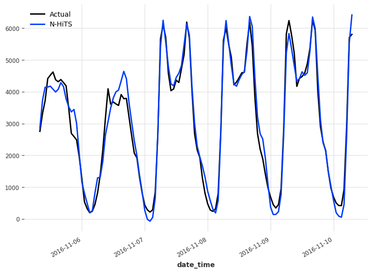
We can visualize the predictions of N-HiTS in the figure below.

test.plot(label='Actual')
pred_nhits.plot(label='N-HiTS')

Then, we simply print out the MAE.

mae_nhits = mae(test, pred_nhits)

print(mae_nhits)

This prints a MAE of 266. Again, we do not beat the baseline, but this is a notable improvement over N-BEATS, as shown below.

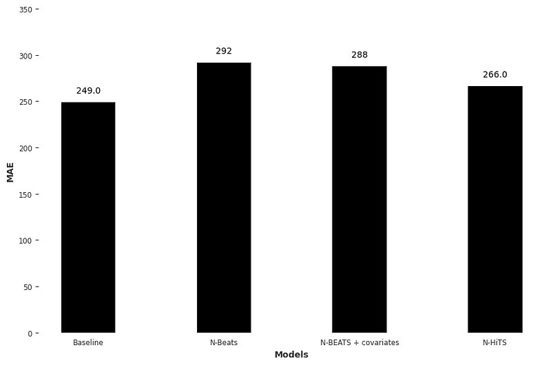
Again, the results are underwhelming since the baseline still outperforms N-HiTS. However, keep in mind that we are working with a small and simple dataset. I only took a sample of the full dataset, and it might that this particular sample if especially repetitive, which explains why the baseline is so good.

Still, you now know how N-HiTS works and how to apply it in a forecasting project!

Conclusion

N-HiTS is the latest development in time series forecasting models, and it was shown to consistently outperform N-BEATS. 

N-HiTS builds upon N-BEATS by adding a MaxPool layer at each block. This subsamples the series and allows each stack to focus on either short-term or long-term effects, depending on the kernel size. Then, the partial predicttions of each stacks are combined using hierarchical interpolation.

This results in N-HiTS being a lighter model with more accurate predictions on long horizons.

I hope that you enjoyed the read and that you learned something new!

Cheers 🍺

Support me

Enjoying my work? Show your support with Buy me a coffee, a simple way for you to encourage me, and I get to enjoy a cup of coffee! If you feel like it, just click the button below 👇