The Easiest Way to Forecast Time Series Using N-BEATS

If, like me, you are interested in time series forecasting, chances are that you stumbled on the model N-BEATS. The model promises state-of-the-art results using a pure deep learning architecture. In other words, it does not need time-series specific components, like trend or seasonality.

Chances are that you read the 2020 paper on N-BEATS written by Oreshkin et al. Although very informative, this paper is not an easy read, and you being here probably means that you agree with me.

So, in this article, I will first explain N-BEATS using more intuition and less equations. Then, I will apply it, using Python, on a real-life forecasting scenario and evaluate its performance.

Let’s get started!

Learn the latest time series analysis techniques with my free time series cheat sheet in Python! Get the implementation of statistical and deep learning techniques, all in Python and TensorFlow!

Understanding N-BEATS

N-BEATS stands for Neural Basis Expansion Analyis for Interpretable Time Series.

As the name suggests, the core functionality of N-BEATS lies in basis expansion. So before diving right into the model’s architecture, let’s first clarify what basis expansion is.

Basis expansion

Basis expansion is a method of augmenting our data. It is often done in order to model non-linear relationships.

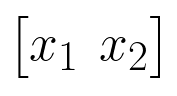
A common basis expansion is polynomial basis expansion. For example, suppose that we have only two features, as shown below.

Then, if we do a polynomial basis expansion of degree 2, our feature set becomes:

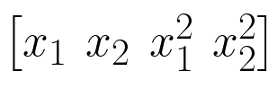
As you can see, the result of the polynomial basis expansion of degree 2 is that we simply added the square of our features to the feature set. 

Therefore, this means that we can now fit a second-degree polynomial model to our data, effectively modeling non-linear relationships!

This is basically what happens in Excel when you fit a linear trend or a polynomial curve to your data.

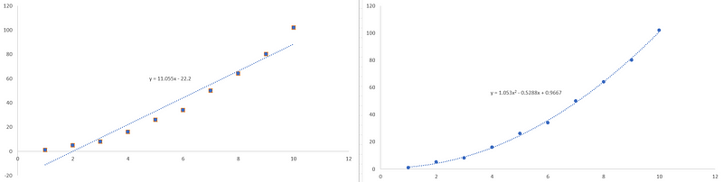
Looking at the figure above, we can see that when we do not perform basis expansion, we only a have a straight line, as shown on the left. However, on the right, once we performed a polynomial basis expansion of degree 2, we then get a quadratic model that if a much better fit to our data.

Of course, basis expansion is not limited to polynomials; we can do logarithms, powers, etc. The main takeaway is that basis expansion is used to augment our set of features in order to model non-linear relationships.

In the case of N-BEATS, the basis expansion is not set by us. Instead, the model is trained to find the best basis expansion method in order to fit the data and make predictions. In other words, we let the neural network find the best data augmentation method to fit our dataset, hence the name: neural basis expansion.

Now that we are comfortable with the concept of basis expansion, let’s move on to the architecture of the model.

The architecture of N-BEATS

There were three key principles in designing the architecture of N-BEATS:

1. The base architecture should be simple and generic, yet expressive
2. The architecture should not rely on time-series-specific components (like trend or seasonality)
3. The architecture can be extendable to make the output interpretable

Following these considerations, the creators of N-BEATS designed the model like this:

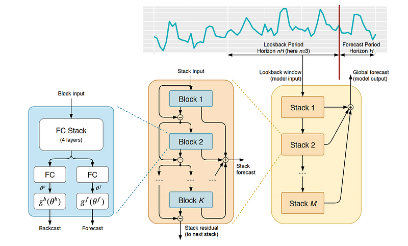
There is a lot of information to absorb from the picture above, so let’s go step by step.

Looking a the top right of the picture, we can see a time series being split between a lookback period and a forecast period. The lookback period is fed to the model, while the forecast period contains the actual values that allows us to evaluate the predictions of our model.

Notice that the input sequence has a length that is a multiple of the forecast length. Therefore, for a forecast horizon of length H, the input sequence should have a length ranging from 2H to 6H typically.

Then, going from right to left in the figure above, we see that N-BEATS (yellow rectangle on the right) is made of layered stacks, which are themselves made of blocks (middle orange rectangle), and we can see how each block is constructed (blue rectangle on the left).

We can see that a block is made of four fully connected layers. This network produces two things: a forecast and a backcast. The forecast is simply a prediction of future values, whereas a backcast is a value coming from the model that we can immediately compare to the input sequence and evaluate the fit of the model.

Note that it is at the block level that the network finds the expansion coefficients (denoted as theta in the diagram) and then the basis expansion is performed (denoted as the function g in the diagram).

In this architecture, only the first block gets the actual input sequence. The following block then gets the residuals coming from the first block. This means that only the information that was not captured by the first block is passed on the next. 

This results in a sequential treatment of the input sequence where each block is trying to capture information that was missed by the previous one.

Combining different blocks together then gives us a stack, which outputs a partial prediction. We then add more stacks to the model, and each stack will output its partial prediction. The combination of each partial prediction then results in the final forecast.

Making the model interpretable

At this point, we understand the inner workings of N-BEATS, but how exactly is this model interpretable?

Right now, it is not. The function responsible for the basis expansion, denoted as g in the diagram, is a learnable function. This means that we let the neural network design a problem-specific function to get the best results.

However, it is possible to constrain the function g to something that we can understand. In time series forecasting, we often use elements like trend and seasonality to inform our forecasts, and we can force the function g to express a trend component or a seasonality component. 

To represent the trend, we use a polynomial basis. To represent seasonality, we use a Fourier basis.

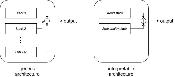
Therefore, in the interpretable version of the architecture, we force the model to have only two stacks: one stack specializes in forecasting a trend component, and the other specializes in forecasting a seasonal component. Then, each prediction is combined to form a final output.

The difference between the generic and interpretable architecture is shown below.

Wrapping up

To summarize, N-BEATS has two configurations. The generic configuration allows the model to find the optimal basis expansion that is specific to our problem. The interpretable configuration forces a stack to specialize in forecasting the trend, and the other stack the seasonality.

The residual connections in the network allows to the model to capture information that was missed by previous blocks. Finally, the combination of the partial prediction of each stack is combined to obtain the final prediction.

I hope I managed to make N-BEATS fairly easy to understand. Now, let’s move on to actually applying N-BEATS in a forecasting project using Python.

Forecasting with N-BEATS

We are now ready to apply the N-BEATS model in a forecasting project. Here, we will predict the hourly Interstate 94 Westbound traffic volume.

We will use the Darts library for this project, as it makes it very easy to apply state-of-the-art models, like N-BEATS, in time series applications. 

All code is in Python and you can grab the full source code, as well as the dataset, on GitHub.

Let’s go!

Read the data

Of course, every project starts off with importing the necessary libraries.

import pandas as pd
import numpy as np
import datetime
import matplotlib.pyplot as plt

from darts import TimeSeries

import warnings
warnings.filterwarnings('ignore')

Then, we actually read our data and store it in a DataFrame.

df = pd.read_csv('data/daily_traffic.csv')

Since we are working with Darts, we will go from DataFrame to a TimeSeries object, which is the fundamental object in Darts. Every model in Darts must have a TimeSeries object as input, and it outputs a TimeSeries object as well.

series = TimeSeries.from_dataframe(df, time_col='date_time')

Now, we can easily visualize our data using the plot method.

series.plot()

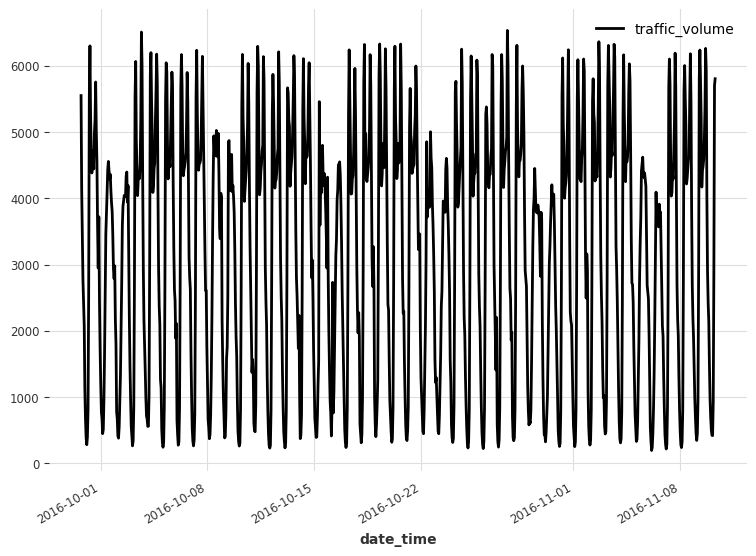
Looking at the figure above, we already identify that we have two seasonal periods: weekly and daily. Clearly, there are more cars on the road during the day than at night, and there are more cars during the week than on the weekend.

This can actually be verified using Darts. It comes with a check_seasonality function that can tell us if a seasonal period has statistical significance.

In this case, since we have hourly data, a daily seasonality has a period of 24 (24 hours in a day), and a weekly seasonality has a period of 168 (24*7 hours in a week).

So, let’s make sure that both seasonal periods are significant.

from darts.utils.statistics import check_seasonality

is_daily_seasonal, daily_period = check_seasonality(series, m=24, max_lag=400, alpha=0.05)
is_weekly_seasonal, weekly_period = check_seasonality(series, m=168, max_lag=400, alpha=0.05)

print(f'Daily seasonality: {is_daily_seasonal} - period = {daily_period}')
print(f'Weekly seasonality: {is_weekly_seasonal} - period = {weekly_period}')

The code block above will print that both seasonal periods are significant, and we will later how we can encode that information to feed it to our model.

Split the data

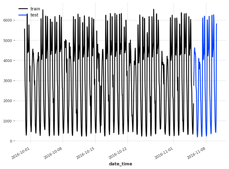
A natural step in a forecasting project to split our data into a training and test set. In this case, we reserve the last five days of data for the test set, and use the rest for training.

train, test = series[:-120], series[-120:]

train.plot(label='train')
test.plot(label='test')

Baseline model

Before using N-BEATS it is good to have a baseline model first. This is a simple model that serves as a benchmark to determine if a more complex model is actually better.

A baseline model usually relies on simple statistics or a simple heuristic. In this case, a naive forecasting method can be to simply repeat the last season. Here, since we have two seasonal periods, we will use the weekly seasonality, to consider that traffic volume is lower on the weekends.

from darts.models.forecasting.baselines import NaiveSeasonal

naive_seasonal = NaiveSeasonal(K=168)
naive_seasonal.fit(train)

pred_naive = naive_seasonal.predict(120)

In the code block above, we simply take the last week of data in the training set and repeat it into the future. Of course, since our forecast horizon has only five days instead of seven, we truncate the predictions at the fifth day.

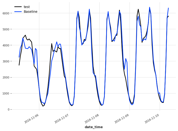
Below, we can visualize the forecasts coming from the baseline model.

test.plot(label='test')
pred_naive.plot(label='Baseline')

Then, we evaluate the performance of the baseline using the mean absolute error (MAE).

from darts.metrics import mae

naive_mae = mae(test, pred_naive)

print(naive_mae)

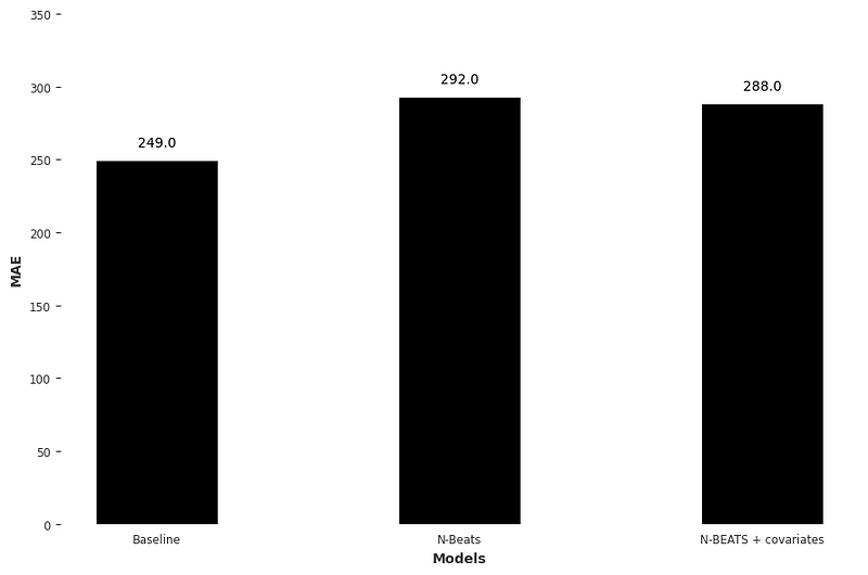
This gives us a MAE of 249, and it is thus the score that we try to beat using N-BEATS.

N-BEATS without covariates

We finally reached the point where we apply N-BEATS to our problem.

We know that we have two seasonal periods, but let’s try N-BEATS without giving it that information. We will let the model work on its own, before we help it out.

We start off by importing N-BEATS and a data scaler to speed up the training of the model.

from darts.models import NBEATSModel
from darts.dataprocessing.transformers import Scaler

We then scale our data between 1 and 0. Note that we fit the scaler on the training set only, because the model is not supposed to have information coming from the test set.

train_scaler = Scaler()
scaled_train = train_scaler.fit_transform(train)

Then, we initialize the N-BEATS model. The input length will contain a full week of data, and the model will output 24h of data. In this case, we use the generic architecture.

nbeats = NBEATSModel(
    input_chunk_length=168, 
    output_chunk_length=24,
    generic_architecture=True,
    random_state=42)

Now, we simply fit the model on the scaled training set.

nbeats.fit(
    scaled_train,
    epochs=50)

Once the model is done training, we can forecast over the horizon of the test set. Of course, the predictions are scaled as well, so we need to reverse the transformation.

scaled_pred_nbeats = nbeats.predict(n=120)

pred_nbeats = train_scaler.inverse_transform(scaled_pred_nbeats)

Finally, we evaluate the performance of N-BEATS.

mae_nbeats = mae(test, pred_nbeats)

print(mae_nbeats)

This gives a MAE of 292, which is higher than the baseline. This means that N-BEATS does not perform better than our naive predictions.

So, let’s add covariates to the model to see if we can improve its performance.

N-BEATS with covariates

Earlier in the article, we determined that there are two seasonal periods that are significant in our time series. We can encode that information and pass it to the model as covariates. 

In other words, we add two features to the model that tells it where we are during the day and during the week. That way, the model learn that weekends have lower traffic volume, and that traffic is lower at night than during the day.

Darts conveniently comes with a an easy to achieve this using datetime_attribute_timeseries .

from darts import concatenate
from darts.utils.timeseries_generation import datetime_attribute_timeseries as dt_attr

cov = concatenate(
    [dt_attr(series.time_index, 'day', dtype=np.float32), dt_attr(series.time_index, 'week', dtype=np.float32)],
    axis='component'
)

We then scale the covariates too to feed it to the model.

cov_scaler = Scaler()
scaled_cov = cov_scaler.fit_transform(cov)

Note that we do not need to split the covariates into a training and test set, because Darts will automatically make the appropriate split during training.

Now, we repeat the process of initializing N-BEATS and fitting it. This time, we pass the covariates as well.

nbeats_cov = NBEATSModel(
    input_chunk_length=168, 
    output_chunk_length=24,
    generic_architecture=True,
    random_state=42)

nbeats_cov.fit(
    scaled_train,
    past_covariates=scaled_cov,
    epochs=50
)

Once the model is trained, we generate the predictions. Remember to reverse the transformation again, since the predictions are scaled between 0 and 1.

scaled_pred_nbeats_cov = nbeats_cov.predict(past_covariates=scaled_cov, n=120)

pred_nbeats_cov = train_scaler.inverse_transform(scaled_pred_nbeats_cov)

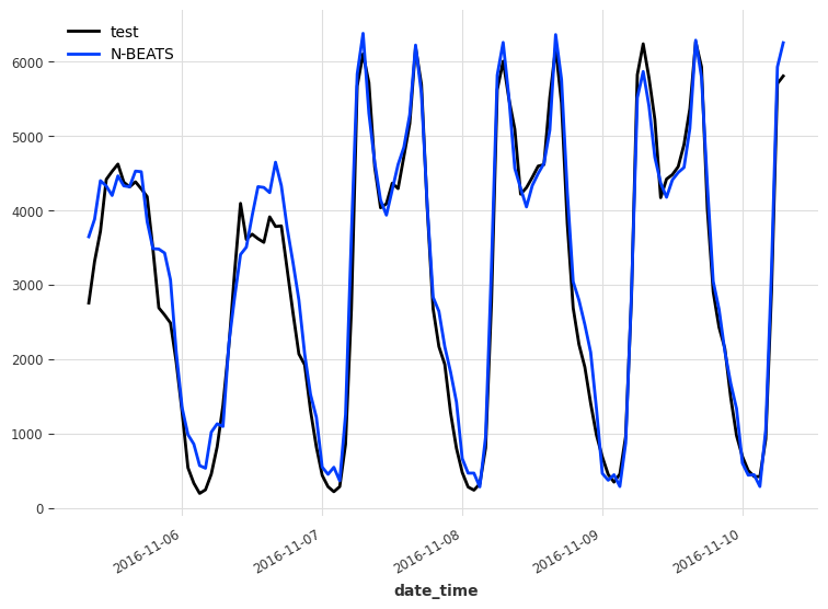
We can also visualize our predictions with the following code block.

test.plot(label='test')
pred_nbeats.plot(label='N-BEATS')

Again, we evaluate the model’s performance using the MAE.

mae_nbeats_cov = mae(test, pred_nbeats_cov)

print(mae_nbeats_cov)

This gives us a MAE of 288. This is better than not using covariates, but still worse than the baseline model.

A note on the results

The results obtained are less than exciting, but take them with a grain salt. Keep in mind that we are working with a fairly small and simple dataset. It might be that the sample I took from the full dataset is simply repetitive by nature, which explains why the baseline is so good.

Nevertheless, you now know how to implement N-BEATS in a forecasting project and you can also appreciate the importance of having a baseline model.

Conclusion

N-BEATS is a state-of-the-art deep learning model for time series forecasting that relies on the principle of basis expansion. The model can learn problem-specific functions for basis expansion, or we can constrain them to have interpretable outputs.

I hope you enjoyed the read and that you learned something new!

Cheers 🍺

Support me

Enjoying my work? Show your support with Buy me a coffee, a simple way for you to encourage me, and I get to enjoy a cup of coffee! If you feel like it, just click the button below 👇