TSMixer: The Latest Forecasting Model by Google

The field of time series forecasting continues to be in effervescence, with many important recent contributions like N-HiTS, PatchTST, TimesNet and of course TimeGPT.

In the meantime, the Transformer architecture unlocked unprecedented performance in the field of natural language processing (NLP), but that is not true for time series forecasting.

In fact, many Transformer-based model were proposed like Autoformer, Informer, FEDformer, and more. Those models are often very long to train and it turns out that simple linear models outperform them on many benchmark datasets (see Zheng et al., 2022).

Tot that point, in September 2023, researchers from Google Cloud AI Research proposed TSMixer, a Multi-layer Perceptron (MLP) based model that focuses on mixing time and feature dimensions to make better predictions.

In their paper TSMixer: An All-MLP Architecture for Time Series Forecasting, the authors demonstrate that this model achieves state-of-the-art performance on many benchmark datasets, while remaining simple to implement.

In this article, we first explore the architecture of TSMixer to understand its inner workings. Then, we implement the model in Python and run our own experiment to compare its performance to N-HiTS.

For more details on TSMixer, make sure to read the original paper.

Learn the latest time series analysis techniques with my free time series cheat sheet in Python! Get the implementation of statistical and deep learning techniques, all in Python and TensorFlow!

Let’s get started!

Explore TSMixer

When it comes to forecasting, we intuitively know that using cross-variate information can help make better predictions.

For example, weather and precipitation are likely to have an impact on the number of visitors to an amusement park. Likewise, the days of the week and holidays will also have an impact.

Therefore, it would make sense to have models that can leverage information from covariates and other features to make predictions.

This is what motivated the creation of TSMixer. As simple univariate linear models were shown to outperform more complex architectures (see Zheng et al., 2022), TSMixer now extends the capabilities of linear models by adding cross-variate feed-forward layers.

Therefore, we now get a linear model capable of handling multivariate forecasting that can leverage information from covariates and other static features.

Architecture of TSMixer

The general architecture is shown in the figure below.

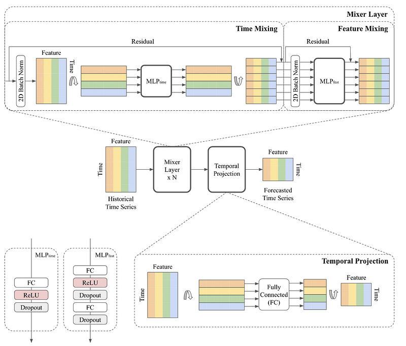
Since TSMixer is simply extending linear models, its architecture is fairly straightforward, since it is entirely MLP-based.

From the figure above, we can see that the model mainly consists of two steps: a mixer layer and a temporal projection.

Let’s explore each step in more detail.

Mixer layer

This is where time mixing and feature mixing occurs, hence the name TSMixer.

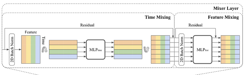
In the figure above, we see that for time mixing, the MLP consists of a fully connected layer, followed by the ReLU activation function, and a dropout layer.

The input, where rows represent time and columns represent features, is transposed so the MLP is applied on the time domain and shared across all features. This unit is responsible for learning temporal patterns.

Before leaving the time mixing unit, the matrix is transposed again, and it is sent to the feature mixing unit.

The feature mixing unit, then consists of two MLPs. Since it is applied in the feature domain, it is shared across all time steps. Here, there is no need to transpose, since the features are already on the horizontal axis.

Notice that in both mixers, we have normalization layers and residual connections. The latter help the model learn deeper representations of the data while keeping the computational cost reasonable, while normalization is a common technique to improve the training of deep learning models.

Once that mixing is done, the output is sent to the temporal projection step.

Temporal projection

The temporal projection step is what generates the predictions in TSMixer.

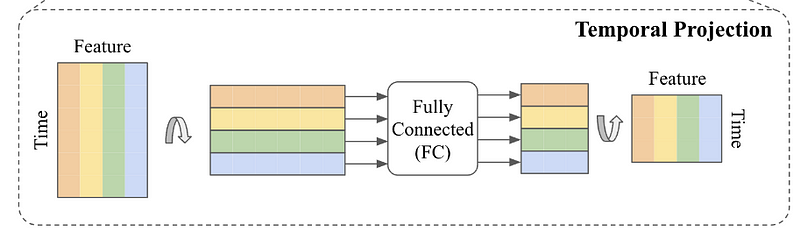
Here, the matrix is again transposed and sent through a fully connected layer to generate predictions. The final step is then to transpose that matrix again to have the features on the horizontal axis, and the time steps on the vertical axis.

Now that we understand how TSMixer works, let’s implement it in Python and test it ourselves.

Implement TSMixer

To my knowledge, TSMixer is not implemented in common time series libraries in Python, like Darts or Neuralforecast. Therefore, I will adapt the original implementation to my experiment for this article.

The original implementation is available in the repository of Google Research.

The complete code for this experiment is available on GitHub.

Read and format the data

The hardest part in applying deep learning models for time series forecasting is arguably formatting the dataset to be fed into the neural network.

So, the first step is create a DataLoader class that handles all the transformations of the dataset. This class is initialized with the batch size, the input sequence length, the output sequence length (the horizon) and a slice object for the targets.

import pandas as pd
import numpy as np
import matplotlib.pyplot as plt
import tensorflow as tf
from sklearn.preprocessing import StandardScaler

class DataLoader:

  def __init__(self, batch_size, seq_len, pred_len):
    self.batch_size = batch_size
    self.seq_len = seq_len
    self.pred_len = pred_len
    self.target_slice = slice(0, None)

    self._read_data()

Then, we add a method to read and scale the data. Here, we use the electricity transformer dataset Etth1, publicly available on GitHub under the Creative Commons Attribute Licence.

def _read_data(self):

    filepath = ('data/ETTh1_original.csv')

    df_raw = pd.read_csv(filepath)
    df = df_raw.set_index('date')

    # split train/valid/test
    n = len(df)
    train_end = int(n * 0.7)
    val_end = n - int(n * 0.2)
    test_end = n

    train_df = df[:train_end]
    val_df = df[train_end - self.seq_len : val_end]
    test_df = df[val_end - self.seq_len : test_end]

    # standardize by training set
    self.scaler = StandardScaler()
    self.scaler.fit(train_df.values)

    def scale_df(df, scaler):
      data = scaler.transform(df.values)
      return pd.DataFrame(data, index=df.index, columns=df.columns)

    self.train_df = scale_df(train_df, self.scaler)
    self.val_df = scale_df(val_df, self.scaler)
    self.test_df = scale_df(test_df, self.scaler)
    self.n_feature = self.train_df.shape[-1]

In the code block above, note that it is crucial to scale our data to improve the model’s training time. Also note that we fit the scaler on the training set only to avoid data leakage in the validation and test sets.

Then, we create two methods for splitting the windows of data into inputs and labels, and then create a dataset that can be fed to a Keras neural network.

def _split_window(self, data):
    inputs = data[:, : self.seq_len, :]
    labels = data[:, self.seq_len :, self.target_slice]

    inputs.set_shape([None, self.seq_len, None])
    labels.set_shape([None, self.pred_len, None])
    return inputs, labels

  def _make_dataset(self, data, shuffle=True):
    data = np.array(data, dtype=np.float32)
    ds = tf.keras.utils.timeseries_dataset_from_array(
        data=data,
        targets=None,
        sequence_length=(self.seq_len + self.pred_len),
        sequence_stride=1,
        shuffle=shuffle,
        batch_size=self.batch_size,
    )
    ds = ds.map(self._split_window)
    return ds

Finally, we complete the DataLoader class with methods to inverse transform the predictions and to generate the training, validation and test sets.

  def inverse_transform(self, data):
    return self.scaler.inverse_transform(data)

  def get_train(self, shuffle=True):
    return self._make_dataset(self.train_df, shuffle=shuffle)

  def get_val(self):
    return self._make_dataset(self.val_df, shuffle=False)

  def get_test(self):
    return self._make_dataset(self.test_df, shuffle=False)

The complete DataLoader class is shown below:

class DataLoader:

  def __init__(self, batch_size, seq_len, pred_len):
    self.batch_size = batch_size
    self.seq_len = seq_len
    self.pred_len = pred_len
    self.target_slice = slice(0, None)

    self._read_data()

  def _read_data(self):

    filepath = ('data/ETTh1_original.csv')

    df_raw = pd.read_csv(filepath)
    df = df_raw.set_index('date')

    # split train/valid/test
    n = len(df)
    train_end = int(n * 0.7)
    val_end = n - int(n * 0.2)
    test_end = n

    train_df = df[:train_end]
    val_df = df[train_end - self.seq_len : val_end]
    test_df = df[val_end - self.seq_len : test_end]

    # standardize by training set
    self.scaler = StandardScaler()
    self.scaler.fit(train_df.values)

    def scale_df(df, scaler):
      data = scaler.transform(df.values)
      return pd.DataFrame(data, index=df.index, columns=df.columns)

    self.train_df = scale_df(train_df, self.scaler)
    self.val_df = scale_df(val_df, self.scaler)
    self.test_df = scale_df(test_df, self.scaler)
    self.n_feature = self.train_df.shape[-1]

  def _split_window(self, data):
    inputs = data[:, : self.seq_len, :]
    labels = data[:, self.seq_len :, self.target_slice]

    inputs.set_shape([None, self.seq_len, None])
    labels.set_shape([None, self.pred_len, None])
    return inputs, labels

  def _make_dataset(self, data, shuffle=True):
    data = np.array(data, dtype=np.float32)
    ds = tf.keras.utils.timeseries_dataset_from_array(
        data=data,
        targets=None,
        sequence_length=(self.seq_len + self.pred_len),
        sequence_stride=1,
        shuffle=shuffle,
        batch_size=self.batch_size,
    )
    ds = ds.map(self._split_window)
    return ds

  def inverse_transform(self, data):
    return self.scaler.inverse_transform(data)

  def get_train(self, shuffle=True):
    return self._make_dataset(self.train_df, shuffle=shuffle)

  def get_val(self):
    return self._make_dataset(self.val_df, shuffle=False)

  def get_test(self):
    return self._make_dataset(self.test_df, shuffle=False)

Then, we can simply initialize an instance of the DataLoader class to read our dataset and create the relevant sets of data.

Here, we use a horizon of 96, an input sequence length of 512, and a batch size of 32.

data_loader = DataLoader(batch_size=32, seq_len=512, pred_len=96)

train_data = data_loader.get_train()
val_data = data_loader.get_val()
test_data = data_loader.get_test()

Now that the data is ready, we can build the TSMixer model.

Build TSMixer

Building TSMixer is fairly easy, as the model consists only of MLPs. Let’s bring back its architecture so we can reference it as we build the model.

First, we must take care of the Mixer Layer, which consists of:

• batch normalization
• transpose the matrix
• feed to a fully connected layer with a ReLu activation
• transpose again
• dropout layer
• and add the residuals at the end

This is translated to code like so:

from tensorflow.keras import layers

def res_block(inputs, norm_type, activation, dropout, ff_dim):

  norm = layers.BatchNormalization

  # Time mixing
  x = norm(axis=[-2, -1])(inputs)
  x = tf.transpose(x, perm=[0, 2, 1])  # [Batch, Channel, Input Length]
  x = layers.Dense(x.shape[-1], activation='relu')(x)
  x = tf.transpose(x, perm=[0, 2, 1])  # [Batch, Input Length, Channel]
  x = layers.Dropout(dropout)(x)
  res = x + inputs

Then, we add the portion for feature mixing which has:

• batch normalization
• a dense layer
• a dropout layer
• another dense layer
• another dropout layer
• and add the residuals to make the residual connection

  # Feature mixing
  x = norm(axis=[-2, -1])(res)
  x = layers.Dense(ff_dim, activation='relu')(x)  # [Batch, Input Length, FF_Dim]
  x = layers.Dropout(0.7)(x)
  x = layers.Dense(inputs.shape[-1])(x)  # [Batch, Input Length, Channel]
  x = layers.Dropout(0.7)(x)
  return x + res

That’s it! The full function for the Mixer Layer is shown below:

from tensorflow.keras import layers

def res_block(inputs, ff_dim):

  norm = layers.BatchNormalization

  # Time mixing
  x = norm(axis=[-2, -1])(inputs)
  x = tf.transpose(x, perm=[0, 2, 1])  # [Batch, Channel, Input Length]
  x = layers.Dense(x.shape[-1], activation='relu')(x)
  x = tf.transpose(x, perm=[0, 2, 1])  # [Batch, Input Length, Channel]
  x = layers.Dropout(0.7)(x)
  res = x + inputs

  # Feature mixing
  x = norm(axis=[-2, -1])(res)
  x = layers.Dense(ff_dim, activation='relu')(x)  # [Batch, Input Length, FF_Dim]
  x = layers.Dropout(0.7)(x)
  x = layers.Dense(inputs.shape[-1])(x)  # [Batch, Input Length, Channel]
  x = layers.Dropout(0.7)(x)
  return x + res

Now, we simply write a function to build the model. We include a for loop to create as many Mixer Layers as we want, and we add the final temporal projection step.

From the figure above, the temporal projection step is simply:

• a transpose
• a pass through a dense layer
• a final transpose

def build_model(
    input_shape,
    pred_len,
    n_block,
    ff_dim,
    target_slice,
):

  inputs = tf.keras.Input(shape=input_shape)
  x = inputs  # [Batch, Input Length, Channel]
  for _ in range(n_block):
    x = res_block(x, norm_type, activation, dropout, ff_dim)

  if target_slice:
    x = x[:, :, target_slice]

  # Temporal projection
  x = tf.transpose(x, perm=[0, 2, 1])  # [Batch, Channel, Input Length]
  x = layers.Dense(pred_len)(x)  # [Batch, Channel, Output Length]
  outputs = tf.transpose(x, perm=[0, 2, 1])  # [Batch, Output Length, Channel])

  return tf.keras.Model(inputs, outputs)

Now, we can run the function to build the model. In this case, we use eight blocks in the Mixer Layer.

model = build_model(
    input_shape=(512, data_loader.n_feature),
    pred_len=96,
    n_block=8,
    ff_dim=64,
    target_slice=data_loader.target_slice
)

Train TSMixer

We are now ready to train the model. 

We use the Adam optimizer with a learning rate of 1e-4. We also implement checkpoints to save the best model and early stopping to stop training if there is no improvements for three consecutive epochs.

tf.keras.utils.set_random_seed(42)

optimizer = tf.keras.optimizers.Adam(1e-4)

model.compile(optimizer, loss='mse', metrics=['mae'])

checkpoint_callback = tf.keras.callbacks.ModelCheckpoint(
    filepath='tsmixer_checkpoints/',
    vebose=1,
    save_best_only=True,
    save_weights_only=True
)

early_stop_callback = tf.keras.callbacks.EarlyStopping(
    monitor='val_loss',
    patience=3
)

history = model.fit(
    train_data,
    epochs= 30,
    validation_data=val_data,
    callbacks=[checkpoint_callback, early_stop_callback]
)

Note that it took 15 minutes to train the model using the CPU only.

Once the model is trained, we can load the best model that was saved by the checkpoint callback.

best_epoch = np.argmin(history.history['val_loss'])

model.load_weights("tsmixer_checkpoints/")

Then, let’s access the predictions for the last window of 96 time steps. Note that the predictions are scaled right now.

predictions = model.predict(test_data)

scaled_preds = predictions[-1,:,:]

Finally, we store both the scaled and inverse transformed predictions in DataFrames to evaluate the performance and plot the predictions later on.

cols = ['HUFL', 'HULL', 'MUFL', 'MULL', 'LUFL', 'LULL', 'OT']

scaled_preds_df = pd.DataFrame(scaled_preds)
scaled_preds_df.columns = cols

preds = data_loader.inverse_transform(scaled_preds)

preds_df = pd.DataFrame(preds)
preds_df.columns = cols

Predict with N-HiTS

To assess the performance of TSMixer, we perform the same training protocol with N-HiTS, as they also support multivariate forecasting.

As a reminder, you can the full code of this experiment on GitHub.

For this section, we use the library NeuralForecast. So the natural first step is to read the data and format it accordingly.

from neuralforecast.core import NeuralForecast
from neuralforecast.models import NHITS

df = pd.read_csv('data/ETTh1_original.csv')

columns_to_melt = ['date', 'HUFL', 'HULL', 'MUFL', 'MULL', 'LUFL', 'LULL', 'OT']

melted_df = df.melt(id_vars=['date'], value_vars=columns_to_melt, var_name='unique_id', value_name='y')

melted_df.rename(columns={'date': 'ds'}, inplace=True)

melted_df['ds'] = pd.to_datetime(melted_df['ds'])

Then, we can initialize N-HiTS and fit on the data.

horizon = 96

models = [
    NHITS(h=horizon, input_size=512, max_steps=30)
]

nf = NeuralForecast(models=models, freq='H')

n_preds_df = nf.cross_validation(
  df=melted_df, 
  val_size=int(0.2*len(df)), 
  test_size=int(0.1*len(df)), 
  n_windows=None)

Then, we extract the predictions for the last 96 time steps only.

df['date'][-96:] = pd.to_datetime(df['date'][-96:])

max_date = df['date'][-96:].max()
min_date = df['date'][-96:].min()

last_n_preds_df = n_preds_df[(n_preds_df['ds'] >= min_date) & (n_preds_df['ds'] <= max_date)]

cols = ['HUFL', 'HULL', 'MUFL', 'MULL', 'LUFL', 'LULL', 'OT']

clean_last_n_preds_df = pd.DataFrame()

for col in cols:
    temp_df = last_n_preds_df[last_n_preds_df['unique_id'] == col].drop_duplicates(subset='ds', keep='first')
    clean_last_n_preds_df = pd.concat([clean_last_n_preds_df, temp_df], ignore_index=True)

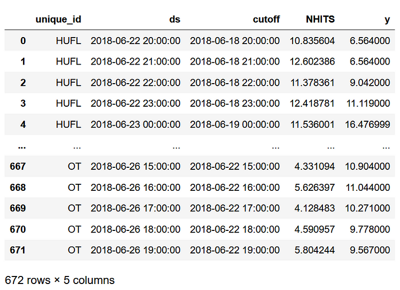
At this point, we have the predictions for each column over the last 96 time steps, as shown below.

Now, we are ready to visualize and measure the performance of our models.

Evaluation

First, let’s visualize the predictions.

For simplicity, we plot only the forecast for the first four series in the dataset.

nhits_preds = pd.read_csv('data/nhits_preds_etth1_h96.csv')
tsmixer_preds = pd.read_csv('data/tsmixer_preds_etth1_h96.csv')

cols_to_plot = ['HUFL', 'HULL', 'MUFL', 'MULL']

fig, axes = plt.subplots(nrows=2, ncols=2, figsize=(12,8))

for i, ax in enumerate(axes.flatten()):
    col = cols_to_plot[i]
    
    nhits_df = nhits_preds[nhits_preds['unique_id'] == col] 
    
    ax.plot(df['date'][-96:], df[col][-96:])
    ax.plot(df['date'][-96:], tsmixer_preds[col], label='TSMixer', ls='--', color='green')
    ax.plot(df['date'][-96:], nhits_df['NHITS'], label='N-HiTS', ls=':', color='black')
    
    ax.legend(loc='best')
    ax.set_xlabel('Time steps')
    ax.set_ylabel('Value')
    ax.set_title(col)
    
plt.tight_layout()
fig.autofmt_xdate()

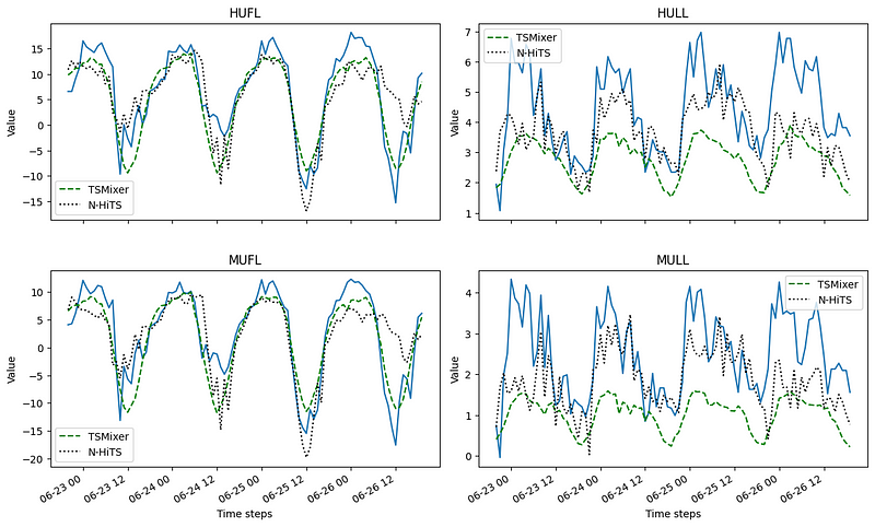
From the figure above, we can see that TSMixer does a pretty good job at forecasting HUFL and MUFL, but it struggles with MULL and HULL. However, N-HiTS seems to be doing fairly good on all series.

Still, the best way to assess the performance is by measuring an error metric. Here, we compute the MAE and MSE.

from sklearn.metrics import mean_absolute_error, mean_squared_error

y_actual = df.drop('date', axis=1)[-96:]

data = {'N-HiTS': 
            [mean_absolute_error(nhits_preds['y'], nhits_preds['NHITS']), 
             mean_squared_error(nhits_preds['y'], nhits_preds['NHITS'])],
       'TSMixer': 
            [mean_absolute_error(y_actual, tsmixer_preds), 
             mean_squared_error(y_actual, tsmixer_preds)]}

metrics_df = pd.DataFrame(data=data)
metrics_df.index = ['mae', 'mse']

metrics_df.style.highlight_min(color='lightgreen', axis=1)

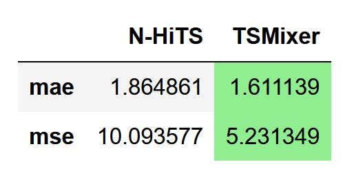
From the figure above, we can see that TSMixer outperforms N-HiTS on the task of multivariate forecasting on a horizon of 96 time steps, since it achieved the lowest MAE and MSE.

While this is not the most extensive experiment, it is interesting to see that kind of performance coming from a rather simple model architecture.

Conclusion

TSMixer is an an all-MLP model specifically designed for multivariate time series forecasting.

It extends the capacity of linear models by adding cross-variate feed-forward layers, enabling the model to achieve state-of-the-art performances on long horizon multivariate forecasting tasks.

While there is no out-of-the-box implementation yet, you now have the knowledge and skills to implement it yourself, as its simple architecture makes it easy for us to do so.

As always, each forecasting problem requires a unique approach and a specific model, so make sure to test TSMixer as well as other models.

Thanks for reading! I hope that you enjoyed it and that you learned something new!

Looking to master time series forecasting? The check out my course Applied Time Series Forecasting in Python. This is the only course that uses Python to implement statistical, deep learning and state-of-the-art models in 16 guided hands-on projects.

Cheers 🍻

Support me

Enjoying my work? Show your support with Buy me a coffee, a simple way for you to encourage me, and I get to enjoy a cup of coffee! If you feel like it, just click the button below 👇

References

Si-An Chen, Chun-Liang Li, Nate Yoder, Sercan O. Arik, Tomas Pfister — TSMixer: An All-MLP Architecture for Time Series Forecasting

Original implementation of TSMixer by the researchers at Google— GitHub