TimesNet: The Latest Advance in Time Series Forecasting

In previous articles, we have explored the latest advances in state-of-the-art forecasting techniques, starting with N-BEATS released in 2020, N-HiTS in 2022, and PatchTST in March 2023. Recall that N-BEATS and N-HiTS rely on the multilayer perceptron architecture, while PatchTST leverages the Transformer architecture.

As of April 2023, a new model was published in the literature, and it achieves state-of-the-art results across multiple tasks in time series analysis, like forecasting, imputation, classification and anomaly detection: TimesNet.

TimesNet was proposed by Wu, Hu, Liu et al in their paper: TimesNet: Temporal 2D-Variation Modeling For General Time Series Analysis.

Unlike previous models, it uses a CNN-based architecture to achieve state-of-the-art results across different tasks, making it a great candidate for a foundation model for time series analysis.

In this article, we explore the architecture and inner workings of TimesNet. Then, we apply the model in a forecasting task, alongside N-BEATS and N-HiTS to complete our own little experiment.

As always, for more details, refer to the original paper.

Learn the latest time series analysis techniques with my free time series cheat sheet in Python! Get the implementation of statistical and deep learning techniques, all in Python and TensorFlow!

Let’s get started!

Explore TimesNet

The motivation behind TimesNet comes from the realization that many real-life time series exhibit mutli-periodicity. This means that variations occur at different periods. 

For example, temperature outside has both a daily and a yearly period. Usually, it is hotter during the day than at night, and hotter during summer than in winter.

Now, those multiple periods overlap and interact with each other, making it difficult to separate and model individually. 

So, the authors of TimesNet propose to reshape the series in a 2D space to model intraperiod-variation and interperiod-variation.

Going back to our weather example, intraperiod-variation would be how the temperature varies within a day, and interperiod-variation would be how the temperature varies from day to day, or from year to year.

With all that in mind, let’s dive into the model’s architecture.

The architecture of TimesNet

Let’s take a look at the architecture of TimesNet.

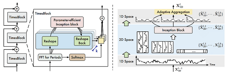
From the figure above, we can see that TimesNet is a stack of multiple TimesBlock with residual connections.

In each TimesBlock, we can see that the series first goes through a fast Fourier transform (FTT) to find the different periods in the data. Then, it is reshaped as a 2D vector and sent to an Inception block where it learns and predicts a 2D representation of the series. Then, this deep representation must be reshaped back to a 1-dimensional vector using adaptive aggregation. 

There is a lot to understand here, so let’s cover each step in more detail.

Capture multi-periodicity

To capture the variations across multiple periods in time series, the authors suggest to transform the 1-dimensional series into a 2-dimensional space to simultaneously model intraperiod and interperiod variations.

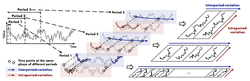
In the figure above, we can see the how the model represents the variations in a 2D space. Inside the red rectangles, we can see the intraperiod-variation, which is how the data changes inside a period. Then, the blue rectangle contains the interperiod-variation, which is how the data changes from period to period.

To better understand that, suppose that we have daily data with a weekly period. The interperiod-variation is how the data changes from Monday, to Tuesday, to Wednesday, and so on.

Then, the interperiod-variation would be how the data varies from Monday in week 1, to Monday in week 2, and from Tuesday in week 1, to Tuesday in week 2. In other words, it is the variation of data in the same phase at different periods.

Those variations are then represented in a 2D space, where the interperiod-variation is vertical, and the intraperiod-variation is horizontal. This allows the model to learn a better representation of the variation in the data. 

Whereas a 1-dimensional vector shows variations between adjacent points, this 2D representation shows variations between adjacent points and adjacent periods, giving a more complete picture of what is happening.

Yet, one question remains: how do we find the periods in our series?

Identify the significant periods in your data

To identify the multiple periods in time series, the model applied the Fast Fourier Transform (FTT).

This is a mathematical operation that transforms a signal into a function of frequency and amplitude.

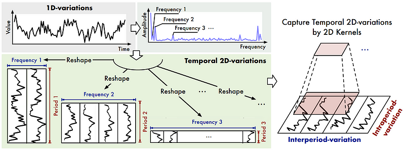
In the figure above, the authors illustrate how FTT is applied. Once we have the frequency and amplitude of each period, the ones with the largest amplitudes are considered to be the most relevant.

For example, here is the result of performing FTT on the Etth1 dataset.

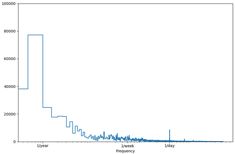
In the figure above, the Fast Fourier Transform allows us to quickly identify a daily and yearly period in our data, since we see higher peaks of amplitude at those periods. 

Once FTT is applied, the user can set a parameter k to select the top-k most important periods, which are the ones with the largest amplitude. 

TimesNet then creates 2D vectors for each period, and those are sent to a 2D kernel to capture the temporal variations.

Inside the TimesBlock

Once the series has gone through the Fourier transform and 2D tensors were created for the top-k periods, the data is sent to the Inception block, as shown in the figure below.

Of course, note that all of the steps that we explored are carried out inside the TimesBlock.

Now, the 2D representation of the data is sent to the Inception block.

The Inception module is the building block of the computer vision model GoogLeNet, published in 2015. 

The main idea of the Inception module is to have an efficient representation of the data by keeping it sparse. That way, we can technically increase the size of a neural network, while keeping it computationally efficient.

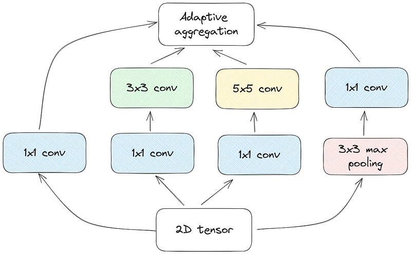
This is achieved by performing various convolutions and pooling operations, and then concatenating everything. In the context of TimesNet, this is how the Inception module looks like.

You might wonder why the authors chose a vision model to treat time series data. 

A simple answer to that is that vision models are particularly good at parsing 2D data, like images.

The other benefit is that the vision backbone can be changed inside TimesNet. While the authors use the Inception block, it can be changed to other vision model backbones, and so TimesNet can also benefit from the advances in computer vision.

Now, one element that separates the Inception module in TimesNet from the inception module in GoogLeNet is the use of adaptive aggregation.

Adaptive aggregation

To perform aggregation, the 2D representation must be reshaped to 1D vectors first.

Then, adaptive aggregation is used, because different periods had different amplitudes, which indicates how important they are.

This is why the output of the FTT is also sent to a softmax layer, so that the aggregation is done using the relative important of each period.

The aggregated data is the output of a single TimesBlock. Then, multiple TimesBlock are stacked with residual connections to create the TimesNet model.

Now that we understand how the TimesNet model works, let’s test it on a forecasting task, alongside N-BEATS and N-HITS.

Forecast with TimesNet

Let’s now apply the TimesNet model on a forecasting task, and compare its performance against N-BEATS and N-HiTS.

For this little experiment, we use the Etth1 dataset released under the Creative Commons Attribution license.

This is a popular benchmark for time series forecasting widely used in literature. It tracks the hourly oil temperature of an electricity transformer which reflects the condition of the equipment.

You can access the dataset and the code on GitHub.

Import libraries and read the data

We start off by importing the required libraries. Here, we use the implementation available in NeuralForecast by Nixtla.

import numpy as np
import pandas as pd
import matplotlib.pyplot as plt

from neuralforecast.core import NeuralForecast
from neuralforecast.models import NHITS, NBEATS, TimesNet

from neuralforecast.losses.numpy import mae, mse

Then, we can read our CSV file.

df = pd.read_csv('data/etth1.csv')

df['ds'] = pd.to_datetime(df['ds'])

df.head()

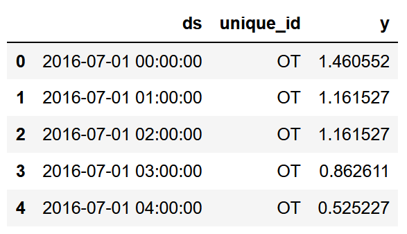
In the figure above, note that the dataset already has the format expected by NeuralForecast. Basically, the package requires three columns:

• a date column labelled as ds
• an id column to label your series, labelled as unique_id
• a value column labelled as y

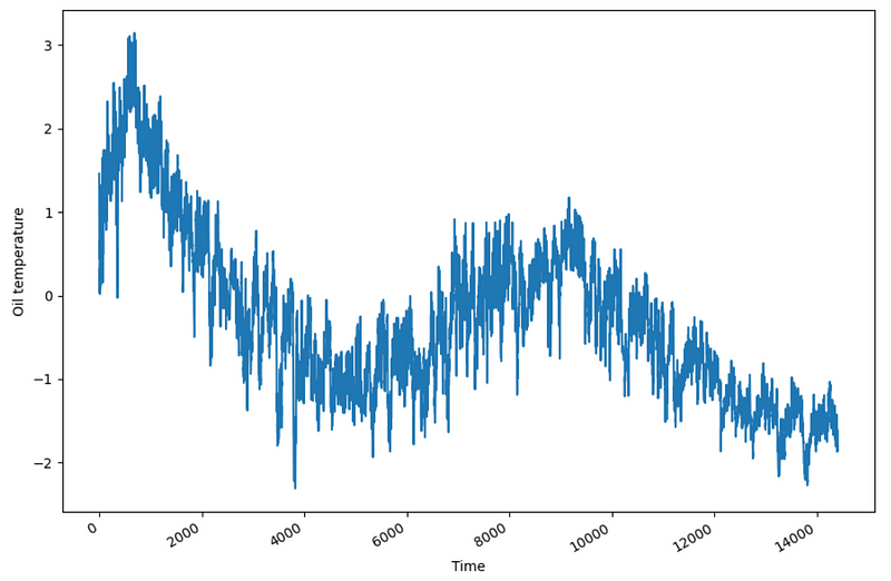
Then, we can plot our series.

fig, ax = plt.subplots()

ax.plot(df['y'])
ax.set_xlabel('Time')
ax.set_ylabel('Oil temperature')

fig.autofmt_xdate()
plt.tight_layout()

Now, we can move on to forecasting.

Forecast

For our experiment, we use a forecasting horizon of 96 hours, which is a common horizon for long-term forecasting in the literature.

We also reserve two windows of 96 time steps to evaluate our models.

First, we define a list of models that we want to use to carry out the forecasting task. Again, we will use N-BEATS, N-HiTS, and TimesNet. 

We will keep the default parameters for all models, and limit the maximum number of epochs to 50. Note that by default, TimesNet will select the top 5 most important periods in our data.

horizon = 96

models = [NHITS(h=horizon,
               input_size=2*horizon,
               max_steps=50),
         NBEATS(h=horizon,
               input_size=2*horizon,
               max_steps=50),
         TimesNet(h=horizon,
                 input_size=2*horizon,
                 max_steps=50)]

Once this is done, we can instantiate the NeuralForecasts object with the list of our models and the frequency of our data, which is hourly.

nf = NeuralForecast(models=models, freq='H')

Then, we run cross-validation so that we have the predictions and the actual values of our dataset. That way, we can evaluate the performance of each model. 

Again, we use two windows of 96 time steps for the evaluation.

preds_df = nf.cross_validation(df=df, step_size=horizon, n_windows=2)

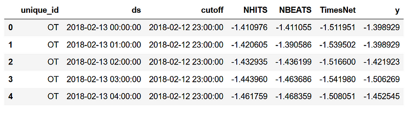
Once the models are trained and predictions are done, we get the DataFrame above. We can see the actual values, as well as the predictions coming from each model that we specified earlier.

We can also easily visualize the predictions against the actual values.

fig, ax = plt.subplots()

ax.plot(preds_df['y'], label='actual')
ax.plot(preds_df['NHITS'], label='N-HITS', ls='--')
ax.plot(preds_df['NBEATS'], label='N-BEATS', ls=':')
ax.plot(preds_df['TimesNet'], label='TimesNet', ls='-.')

ax.legend(loc='best')
ax.set_xlabel('Time steps')
ax.set_ylabel('Oil temperature')

fig.autofmt_xdate()
plt.tight_layout()

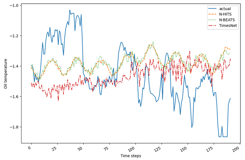
In the figure above, it seems that all models fail to predict the decrease in oil temperature observed in the test set. Also, N-BEATS and N-HiTS have captured some cyclical pattern that is not observed in the predictions of TimesNet.

Still, we need to evaluate the models by calculating the MSE and MAE to determine which model is best.

Evaluation

Now, we simply compute the MAE and MSE to find out which model performed best.

data = {'N-HiTS': [mae(preds_df['NHITS'], preds_df['y']), mse(preds_df['NHITS'], preds_df['y'])],
       'N-BEATS': [mae(preds_df['NBEATS'], preds_df['y']), mse(preds_df['NBEATS'], preds_df['y'])],
       'TimesNet': [mae(preds_df['TimesNet'], preds_df['y']), mse(preds_df['TimesNet'], preds_df['y'])]}

metrics_df = pd.DataFrame(data=data)
metrics_df.index = ['mae', 'mse']

metrics_df.style.highlight_min(color='lightgreen', axis=1)

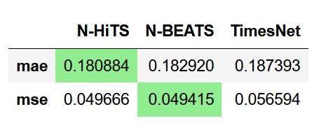
From the figure above, we can see the N-HiTS achives the lowest MAE, while N-BEATS achieves the lowest MSE. 

However, there is a difference of 0.002 in MAE, and a difference of 0.00025 in MSE. Since the difference in MSE is so small, especially considering the error is squared, I would argue that N-HiTS is the champion model for this task.

So, it turns out that TimesNet did not achieve the best performance. However, keep in mind that we just conducted a simple experiment with no hyperparameter optimization, on one dataset only, and on two windows of 96 time steps. 

This is really meant to show you how to work with TimesNet and NeuralForecast, so that you can have another tool in your toolbox to solve your next forecasting problem.

Conclusion

TimesNet is a CNN-based model that leverages the Inception module to achieve state-of-the-art performances on many time series analysis tasks, such as forecasting, classification, imputation and anomaly detection.

As always, each forecasting problem requires a unique approach and a specific model, so make sure to test out TimesNet as well as other models.

Thanks for reading! I hope that you enjoyed it and that you learned something new!

Looking to master time series forecasting? The check out my course Applied Time Series Forecasting in Python. This is the only course that uses Python to implement statistical, deep learning and state-of-the-art models in 16 guided hands-on projects.

Cheers 🍻

Support me

Enjoying my work? Show your support with Buy me a coffee, a simple way for you to encourage me, and I get to enjoy a cup of coffee! If you feel like it, just click the button below 👇

References

Haixu Wu, Tengge Hu, Yong Liu, Hang Zhou, Jianmin Wang and Mingsheng Long — TimesNet: Temporal 2D-Variation Modeling For General Time Series Analysis

Christian Szegedy, Wei Liu, Yangqing Jia, Pierre Sermanet, Scott Reed,
Dragomir Anguelov, Dumitru Erhan, Vincent Vanhoucke, Andrew Rabinovich — Going Deeper With Convolutions