TimeGPT: The First Foundation Model for Time Series Forecasting

The field of time series forecasting is going through a very exciting period. In only the last three years, we have seen many important contributions, like N-BEATS, N-HiTS, PatchTST and TimesNet.

At the same time, large language models (LLMs) have gained a lot of popularity lately, with applications like ChatGPT, as they can adapt to a wide variety of tasks without further training.

Which leads to the question: can foundation models exist for time series like they exist for natural language processing? Is it possible that a large model pre-trained on massive amounts of time series data can then produce accurate predictions on unseen data?

With TimeGPT-1, proposed by Azul Garza and Max Mergenthaler-Canseco, the authors adapt the techniques and architecture behind LLMs to the field of forecasting, successfully building the first time series foundation model capable of zero-shot inference.

In this article, we first explore the architecture behind TimeGPT and how the model was trained. Then, we apply it in a forecasting project to evaluate its performance against other state-of-the-art methods, like N-BEATS, N-HiTS and PatchTST. 

For more details, make sure to read the original paper.

Learn the latest time series analysis techniques with my free time series cheat sheet in Python! Get the implementation of statistical and deep learning techniques, all in Python and TensorFlow!

Let’s get started!

Explore TimeGPT

As mentioned earlier, TimeGPT is a first attempt at creating a foundation model for time series forecasting.

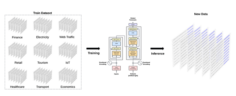
From the figure above, we can see that the general idea behind TimeGPT is to train a model on massive amounts of data from different domains to then produce zero-shot inference on unseen data.

Of course, this method relies on transfer learning, which is the capacity of a model to solve a new task using its knowledge gained during training.

Now, this only works if the model is large enough, and if it is trained on lots of data. 

Training TimeGPT

To that end, the authors trained TimeGPT on more than 100 billion data points all coming from open-source time series data. The dataset spans a wide array of domains, from finance, economics and weather, to web traffic, energy and sales.

Note that the authors do not disclose the sources of public data used to curate 100 billion data points. 

This variety is critical for the success of a foundation model, as it can learn different temporal patterns and therefore generalize better.

For example, we can expect weather data to have a daily (hotter during the day than at night) and yearly seasonality, while car traffic data can have a daily seasonality (more cars on the road during the day than at night) and a weekly seasonality (more cars on the road during the week than on weekends).

To ensure the robustness and generalization capabilities of the model, preprocessing was kept to a minimum. In fact, only missing values were filled, and the rest was kept in its raw form. While the authors do not specify the method for data imputation, I suspect that some kind of interpolation technique was used, like linear, spline or moving average interpolation. 

The model was then trained over multiple days, during which hyperparameters and learning rates were optimized. While the authors do not disclose how many days and GPUs were required for training, we do know that the model is implemented in PyTorch, and it uses the Adam optimizer and a learning rate decay strategy.

Architecture of TimeGPT

TimeGPT leverages the Transformer architecture with self-attention mechanism based on the seminal work of Google and the University of Toronto in 2017.

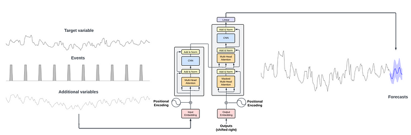
From the figure above, we can see that TimeGPT uses the full encoder-decoder Transformer architecture.

The inputs can consist of a window of historical data, as well as exogenous data, like punctual events or another series. 

The inputs are fed to the encoder portion of the model. The attention mechanism inside the encoder then learns different properties from the inputs. This is then fed to the decoder, which uses the learned information to produce forecasts. Of course, the sequence of predictions ends when it reaches the length of the forecast horizon set by the user.

It is important to note that the authors have implemented conformal predictions in TimeGPT, allowing the model to estimate prediction intervals based on historic errors. 

The capabilities of TimeGPT

TimeGPT comes with a wide array of capabilities considering that it is a first attempt at building a foundation model for time series.

First, with TimeGPT being a pre-trained model, it means that we can generate predictions without training it on our data specifically. Still, it is possible to fine-tune the model to our data.

Second, the model supports exogenous variables to forecast our target, and it can handle multivariate forecasting tasks.

Finally, with the use of conformal prediction, TimeGPT can estimate prediction intervals. This in turn allows the model to perform anomaly detection. Basically, if a data point falls outside of a 99% confidence interval, then the model labels it as an anomaly.

Keep in mind that all those tasks are possible with zero-shot inference, or with some fine-tuning, which is a radical shift in paradigm for the field of time series forecasting.

Now that we have a more solid understanding of TimeGPT, how it works and how it was trained, let’s see the model in action.

Forecast with TimeGPT

Let’s now apply TimeGPT on a forecasting task and compare its performance to other models.

Note that at the time of writing this article, TimeGPT is only accessible by API, and it is in closed beta. I submitted a request and was granted free access to the model for two weeks. To get a token and access the model, you have to visit their website.

As mentioned earlier, the model was trained on 100 billion data points coming from publicly available data. Since the authors do not specify the actual datasets used, I think it is unreasonable to test the model on known benchmark datasets, like ETT or weather, as the model has likely seen this data during training.

Therefore, I compiled and open-sourced my own dataset for this article.

Specifically, I curated the daily views on my blog from January 1st 2020, to October 12th 2023. I also added two exogenous variables: one to signal a day where a new article was published, and the other to flag a day where it is a holiday in the United States, as the majority of my audience lives there.

The dataset is now publicly available on GitHub, and most importantly, we are sure that TimeGPT did not train on this data.

As always, you can access the full notebook on GitHub.

Import libraries and read the data

The natural first step is to import the libraries for this experiment.

import pandas as pd
import numpy as np
import datetime
import matplotlib.pyplot as plt

from neuralforecast.core import NeuralForecast
from neuralforecast.models import NHITS, NBEATS, PatchTST

from neuralforecast.losses.numpy import mae, mse

from nixtlats import TimeGPT

%matplotlib inline

Then, to access the TimeGPT model, we read the API key from a file. Note that I did not assign the API key to an environment variable, because the access was limited to two weeks only.

with open("data/timegpt_api_key.txt", 'r') as file:
        API_KEY = file.read()

Then, we can read the data.

df = pd.read_csv('data/medium_views_published_holidays.csv')
df['ds'] = pd.to_datetime(df['ds'])

df.head()

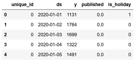
From the figure above, we can see that the format of the dataset is the same as when we work with other open-source libraries from Nixtla. 

We have a unique_id column to label different time series, but in our case, we only have one series. 

The column y represents the daily views on my blog, and published is a simple flag to label a day where a new article was published (1) or no article was published (0). Intuitively, we know that when new content is released, the views usually increase for a period of time. 

Finally, the column is_holiday indicates if there is a holiday or not in the United States. The intuition is that on holidays, fewer people will visit my blog.

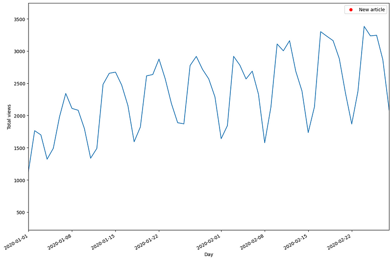
Now, let’s visualize our data and look for discerning patterns.

published_dates = df[df['published'] == 1]

fig, ax = plt.subplots(figsize=(12,8))

ax.plot(df['ds'], df['y'])
ax.scatter(published_dates['ds'], published_dates['y'], marker='o', color='red', label='New article')
ax.set_xlabel('Day')
ax.set_ylabel('Total views')
ax.legend(loc='best')

fig.autofmt_xdate()


plt.tight_layout()

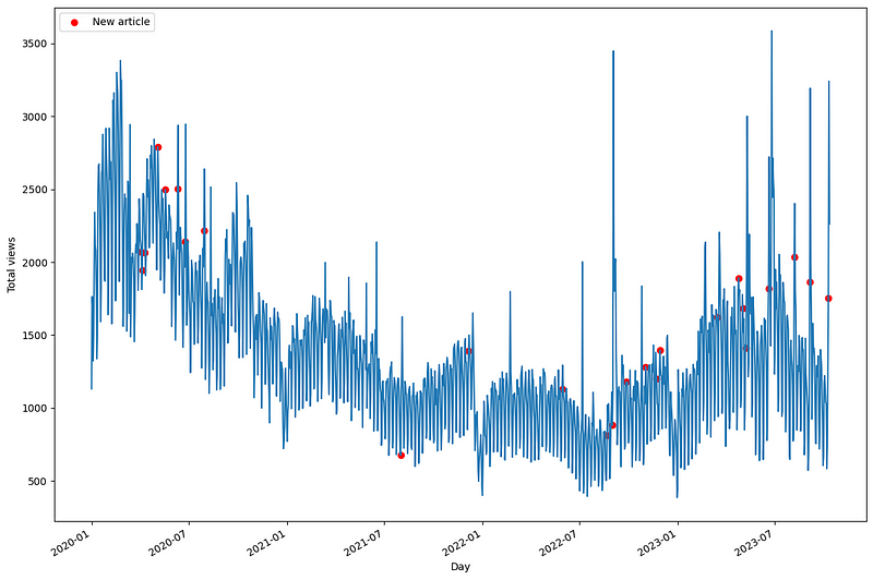
From the figure above, we can already see some interesting behaviour. First, notice that the red dots indicate a new published article, and they are almost immediately followed by peaks in visits.

We also notice less activity in 2021 which is reflected in fewer daily views on my blog. Finally, in 2023, we notice some anomalous peaks in visits after an article is published.

Zooming in on the data, we also uncover a clear weekly seasonality.

From the figure above, we can now see that fewer visitors come to the blog during the weekend than during the week.

With all of that in mind, let’s see how we can work with TimeGPT to make predictions.

Predict with TimeGPT

First, let’s split the dataset into a training set and a test set. Here, I will keep 168 time steps for the test set, which corresponds to 24 weeks of daily data.

train = df[:-168]
test = df[-168:]

Then, we work with a forecast horizon of seven days, as I am interested in predicting the daily views for a full week.

Now, the API does not come with an implementation of cross-validation. Therefore, we create our own loop to generate seven predictions at a time, until we have predictions for the entire test set.

future_exog = test[['unique_id', 'ds', 'published', 'is_holiday']]

timegpt = TimeGPT(token=API_KEY)

timegpt_preds = []

for i in range(0, 162, 7):

    timegpt_preds_df = timegpt.forecast(
        df=df.iloc[:1213+i],
        X_df = future_exog[i:i+7],
        h=7,
        finetune_steps=10,
        id_col='unique_id',
        time_col='ds',
        target_col='y'
    )
    
    preds = timegpt_preds_df['TimeGPT']
    
    timegpt_preds.extend(preds)

In the code block above, notice that we have to pass the future values of our exogenous variables. This is fine, because they are static variables. We know the future dates of holidays, and the blog author personally knows when he plans on publishing an article.

Also note that we fine-tune TimeGPT to our data using the finetune_steps parameter.

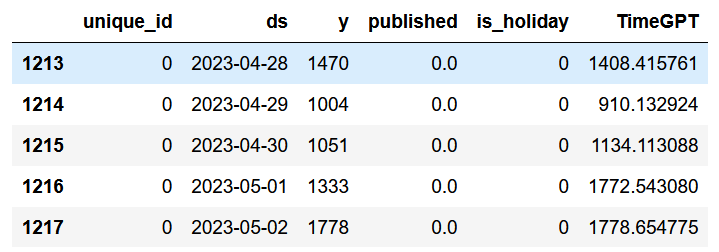
Once the loop is done, we can add the predictions to the test set. Again, TimeGPT generated seven predictions at a time until 168 predictions were obtained, so that we can evaluate its capacity in forecasting the daily views for next week.

test['TimeGPT'] = timegpt_preds

test.head()

Forecasting with N-BEATS, N-HiTS and PatchTST

Now, let’s apply other methods to see if training these models specifically on our dataset can produce better predictions.

For this experiment, as mentioned before, we use N-BEATS, N-HiTS and PatchTST.

horizon = 7

models = [NHITS(h=horizon,
               input_size=5*horizon,
               max_steps=50),
         NBEATS(h=horizon,
               input_size=5*horizon,
               max_steps=50),
         PatchTST(h=horizon,
                 input_size=5*horizon,
                 max_steps=50)]

Then, we initialize the NeuralForecast object and specify the frequency of our data, which is daily in this case.

nf = NeuralForecast(models=models, freq='D')

Then, we run perform cross-validation over 24 windows of 7 time steps to have predictions that align with the test set used for TimeGPT.

preds_df = nf.cross_validation(
    df=df, 
    static_df=future_exog , 
    step_size=7, 
    n_windows=24
)

Then, we can simply add the predictions from TimeGPT to this new preds_df DataFrame to have a single DataFrame with the predictions from all models.

preds_df['TimeGPT'] = test['TimeGPT']

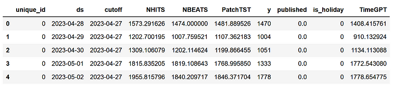
Great! We are now ready to evaluate the performance of each model.

Evaluation

Before measuring performance metrics, let’s visualize the predictions of each model on our test set.

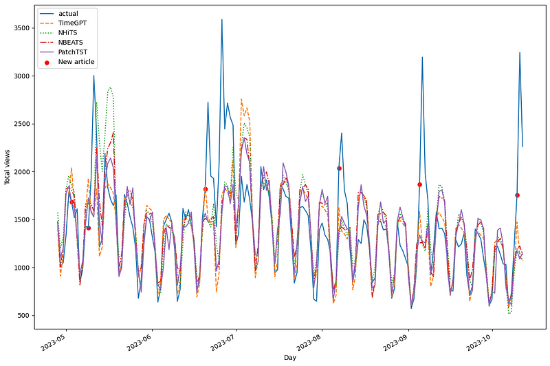
First, we see a lot of overlapping between each model. However, we do notice that N-HiTS predicted two peaks that were not realized in real life. Also, it seems that PatchTST is often under-forecasting. However, TimeGPT seem to generally overlap the actual data quite well.

Of course, the only way to assess each model’s performance is to measure performance metrics. Here, we use the mean absolute error (MAE) and mean squared error (MSE). Also, we round the predictions to whole numbers, as a decimal number makes no sense in the context of daily visitors to a blog.

preds_df = preds_df.round({
    'NHITS': 0,
    'NBEATS': 0,
    'PatchTST': 0,
    'TimeGPT': 0
})

data = {'N-HiTS': [mae(preds_df['NHITS'], preds_df['y']), mse(preds_df['NHITS'], preds_df['y'])],
       'N-BEATS': [mae(preds_df['NBEATS'], preds_df['y']), mse(preds_df['NBEATS'], preds_df['y'])],
       'PatchTST': [mae(preds_df['PatchTST'], preds_df['y']), mse(preds_df['PatchTST'], preds_df['y'])],
       'TimeGPT': [mae(preds_df['TimeGPT'], preds_df['y']), mse(preds_df['TimeGPT'], preds_df['y'])]}

metrics_df = pd.DataFrame(data=data)
metrics_df.index = ['mae', 'mse']

metrics_df.style.highlight_min(color='lightgreen', axis=1)

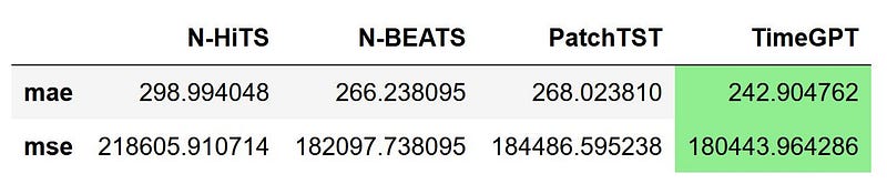
From the figure above, we see that TimeGPT is the champion model as it achieves the lowest MAE and MSE, followed by N-BEATS, PatchTST and N-HiTS.

This is an exciting result, as TimeGPT has never seen this dataset and was only fine-tuned for a few steps. While this is not an exhaustive experiment, I believe it does show a glimpse of the potential foundational models can have in the field of forecasting.

My personal opinion on TimeGPT 

While my short experiment with TimeGPT proved to be exciting, I must point out that the original paper remains vague in many important areas.

Again, we do not know what datasets were used to train and test the model, so we cannot really verify the performance results of TimeGPT, as shown below.

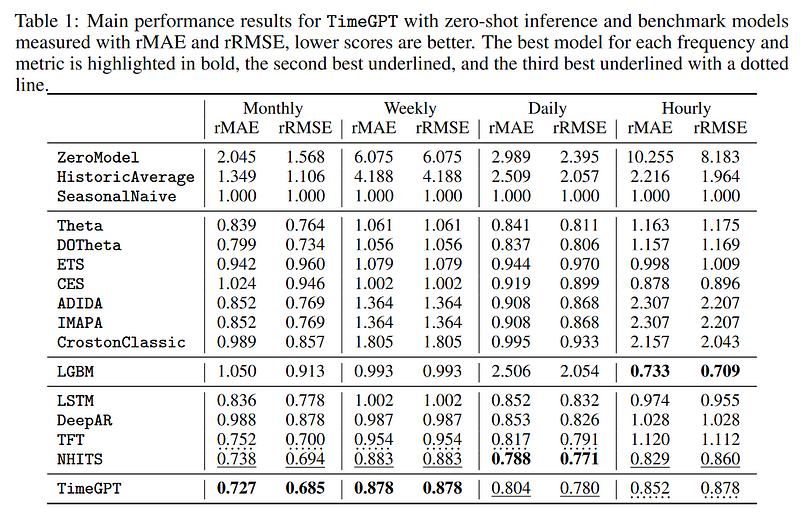
From the table above, we can see that TimeGPT performs best for the monthly and weekly frequencies, with N-HiTS and Temporal Fusion Transformer (TFT) usually ranking 2nd or 3rd. Then again, because we do not know what data was used, we cannot verify these metrics.

There is also a lack of transparency when it comes to how the model was trained and how it was adapted to handle time series data.

I believe that the model is intended for commercial use, which explains why the paper lacks the details to reproduce TimeGPT. There is nothing wrong with that, but the lack of reproducibility of the paper is a concern for the scientific community.

Still, I hope that this sparks new work and research in foundation models for time series, and that we eventually see an open-source version of these models, much like we see it happening for LLMs.

Conclusion

TimeGPT is the first foundation model for time series forecasting. 

It leverages the Transformer architecture and was pre-trained on 100 billion data points to make zero-shot inference on new unseen data.

Combined with the technique of conformal prediction, the model can generate prediction intervals and perform anomaly detection without being trained on a specific dataset.

I still believe that each forecasting problem requires a unique approach, so make sure to test out TimeGPT as well as other models.

Thanks for reading! I hope that you enjoyed it and that you learned something new!

Looking to master time series forecasting? Then check out my course Applied Time Series Forecasting in Python. This is the only course that uses Python to implement statistical, deep learning and state-of-the-art models in 16 guided hands-on projects.

Cheers 🍻

Support me

Enjoying my work? Show your support with Buy me a coffee, a simple way for you to encourage me, and I get to enjoy a cup of coffee! If you feel like it, just click the button below 👇

References

TimeGPT-1 by Azul Garza and Max Mergenthaler-Canseco