Time Series Forecasting with TiDE

In our exploration of the latest advances in the field of time series forecasting, we discovered N-HiTS, PatchTST, TimeGPT and also TSMixer.

While many efforts have been deployed to apply the Transformer architecture for forecasting, it turns out that it achieves a mediocre performance considering the computation requirements.

In fact, simple linear models have been shown to outperform the complex Transformer-based models on many benchmark datasets (see Zheng et al., 2022).

Motivated by that, in April 2023, researchers at Google proposed TiDE: a long-term forecasting model with an encoder-decoder architecture built with Multilayer Perceptrons (MLPs).

In their paper Long-term Forecasting with TiDE: Time-series Dense Encoder, the authors demonstrate that the model achieves state-of-the-art results on numerous datasets when compared to other Transformer-based and MLP-based models, like PatchTST and N-HiTS respectively.

In this article, we first explore the architecture and inner workings of TiDE. Then, we apply the model in Python and use it in our own small forecasting experiment.

For more details on TiDE, make sure to read the original paper.

Learn the latest time series analysis techniques with my free time series cheat sheet in Python! Get the implementation of statistical and deep learning techniques, all in Python and TensorFlow!

Let’s get started!

Explore TiDE

TiDE stands for Time-series Dense Encoder. At its base, this model implements the encoder-decoder concept without the attention mechanism in Transformer-based models.

Instead, it relies on MLPs to achieve faster training and inference times, while achieving good performance.

During training, the model will encode historical data along with covariates. Then, it will decode the learned representation along with known future covariates to make predictions.

Architecture of TiDE

The architecture of TiDE is presented in the figure below.

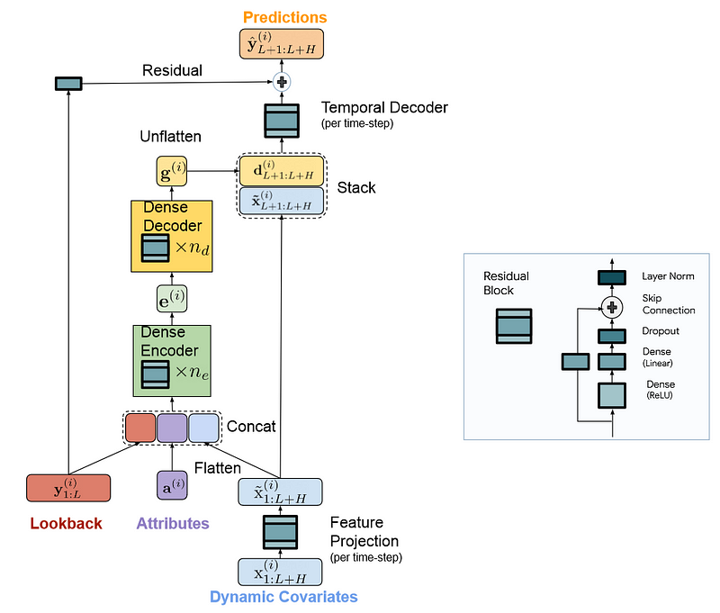
From the figure above, we can see that the model treats each series as an independent channel, meaning that one series along with its covariates are passed at a time.

We also see that there are three main components to the model: an encoder, a decoder and a temporal decoder, and all rely on the residual block architecture.

There is a lot of information in this figure, so let’s explore each component in more detail.

Explore the residual block

As mentioned, the residual block serves as the base layer in TiDE’s architecture.

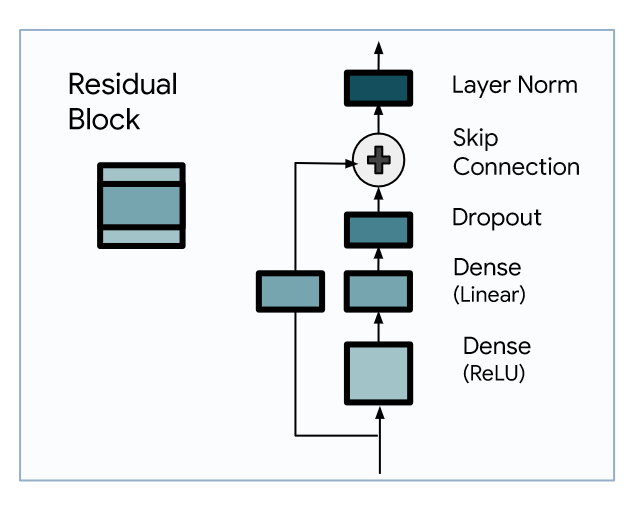
From the figure above, we see that it is an MLP with one hidden layer and a ReLU activation. This is followed by a dropout layer, a skip connection, and a final layer normalization step.

Then, this component is reused across the network to encode, decode and make predictions.

Understand the encoder

During this step, the model maps the past and the covariates of a time series to a dense representation. 

The first step if to carry out feature projection. This is where the residual block is used to map dynamic covariates (exogenous variables varying in time) into a lower dimensional projection. 

Keep in mind that when performing multivariate forecasting, we need the future values of our features. Therefore, the model must treat a look-back window and a horizon sequence. 

These sequences can get very long, so by projecting to a lower dimensional space, we keep the lengths manageable and allow the model to treat longer sequences, both in terms of historical window and horizon of forecast.

The second step, is then to concatenate the past of the series with its attributes and projection of past and future covariates. This is then sent to the encoder, which is simply a stack of residual blocks.

The encoder is thus responsible for learning a representation of the inputs. This can be seen as a learned embedding.

Once done, the embedding is sent to the decoder.

Understand the decoder

Here, the decoder is responsible for taking the learned representation of the encoder and generating predictions.

The first step is the dense decoder, which is also composed of a stack of residual blocks. This takes the encoded information and outputs a matrix to be fed to the temporal decoder.

The decoded output is stacked with projected features to capture direct effects of future covariates. For example, holidays are punctual events that can have important impacts on certain time series. With this residual connection, the model can capture and leverage that information.

The second step is then the temporal decoder, where predictions are generated. Here, it is simply a residual block with an output size of 1, such that we get the predictions for a given time series.

Now that we understand each critical component of TiDE, let’s apply it in a small forecasting project using Python.

Forecast using TiDE

Now, let’s apply TiDE in a small forecasting project and compare its performance to TSMixer. 

Interestingly, TSMixer is also an MLP-based architecture for multivariate forecasting developed by Google researchers, but it was published a month before TiDE. So I think it is interesting to compare both models in a small experiment.

For more details on TSMixer, make sure to read my article entirely dedicated to it.

In this project, we use the Etth1 dataset released under the Creative Commons Attribution license.

This is a popular benchmark for time series forecasting widely used in literature. It tracks the hourly oil temperature of an electricity transformer along with other covariates, making it a great scenario for multivariate forecasting. 

The full source code of this experiment is available on GitHub.

Import libraries and read the data

The natural first step is to import the required libraries for this project and read the data.

While the source code of the original paper of TiDE is publicly available on GitHub, I instead opted to use the implementation available in Darts.

It will provide us with greater flexibility and it comes with hyperparameter optimization capabilities that are not available in the original repository.

So, let’s import darts as well as other standard packages.

import pandas as pd
import numpy as np
import matplotlib.pyplot as plt

from darts import TimeSeries
from darts.datasets import ETTh1Dataset

Then, we can read our data. Luckily for us, Darts comes with standard datasets used across academia, like the Etth1 dataset.

series = ETTh1Dataset().load()

Finally, let’s split our data and reserve the last 96 time steps for the test set. 

train, test = series[:-96], series[-96:]

We are now ready to train our TiDE model.

Train TiDE

To access TiDE, we simply import it from the darts library. We also need to manually scale our data before training. This ensures a faster and more stable training procedure.

from darts.models.forecasting.tide_model import TiDEModel
from darts.dataprocessing.transformers import Scaler

train_scaler = Scaler()
scaled_train = train_scaler.fit_transform(train)

Then, we initialize the model and specify its parameters. Here, I am using the same optimized parameters as presented in the paper for this particular dataset.

tide = TiDEModel(
    input_chunk_length=720, 
    output_chunk_length=96,
    num_encoder_layers=2,
    num_decoder_layers=2,
    decoder_output_dim=32,
    hidden_size=512,
    temporal_decoder_hidden=16,
    use_layer_norm=True,
    dropout=0.5,
    random_state=42)

Then, we can simply fit the model. Note that I only train it on 30 epochs, so feel free to increase that number if you have more time and computing resources available.

tide.fit(
    scaled_train,
    epochs=30
)

Once the model is done training, we can access its predictions. Note that because we scaled the training data, the model also outputs scaled predictions. Therefore, we must reverse the transformation.

scaled_pred_tide = tide.predict(n=96)

pred_tide = train_scaler.inverse_transform(scaled_pred_tide)

Perfect! We can then evaluate the performance of TiDE.

Evaluate the performance

To evaluate our model’s performance, let’s store the predictions and the actual values in a DataFrame.

preds_df = pred_tide.pd_dataframe()
test_df = test.pd_dataframe()

Optionally, we can visualize the predictions. For simplicity, I am only plotting four columns.

cols_to_plot = ['OT', 'HULL', 'MUFL', 'MULL']

fig, axes = plt.subplots(nrows=2, ncols=2, figsize=(12,8))

for i, ax in enumerate(axes.flatten()):
    col = cols_to_plot[i]
        
    ax.plot(test_df[col], label='Actual', ls='-', color='blue')
    ax.plot(preds_df[col], label='TiDE', ls='--', color='green')
    
    ax.legend(loc='best')
    ax.set_xlabel('Date')
    ax.set_title(col)
    
plt.tight_layout()
fig.autofmt_xdate()

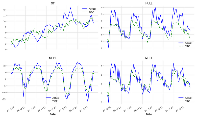
From the figure above, we can see that TiDE does a pretty good job at forecasting each series. 

Of course, the best way to evaluate the performance is to calculate error metrics, so let’s compute the mean absolute error (MAE) and mean squared error (MSE).

from darts.metrics import mae, mse

tide_mae = mae(test, pred_tide)
tide_mse = mse(test, pred_tide)

print(tide_mae, tide_mse)

This gives us a MAE of 1.19 and a MSE of 3.58.

Now, to keep this article at reasonable length, I will not cover the implementation of TSMixer. 

At this moment, there is no ready-to-use implementation of it, so we have to many steps manually. Again, for more details, you can read my article covering TSMixer.

For now, let’s just report the performance of TSMixer for multivariate forecasting on the Etth1 dataset on a horizon of 96 time steps.

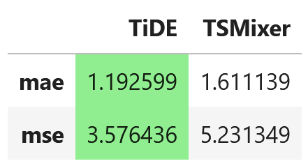
From the figure above, we can see that TiDE achieves the lowest MAE and MSE, meaning that it outperforms TSMixer.

Of course, this is not an extensive experiment, so it does not mean that TiDE is always better than TSMixer. 

Although both models have an MLP-based architecture, it may be that TiDE represents an incremental improvement over TSMixer. Nevertheless, you should always test different models for your particular dataset and find which works best.

Conclusion

TiDE stands for Time-series Dense Encoder, and it is an MLP-based model designed for long-horizon multivariate forecasting.

It relies on the residual block unit to first encode covariates and historical data. Then, it decodes the learned representation and generates forecast. 

Since its only MLPs, it benefits from faster training times and it was demonstrated to still achieve high performances on long-term forecasting tasks.

Of course, each problem is unique, so make sure to test TiDE as well as other models.

Thanks for reading! I hope that you enjoyed it and that you learned something new!

Looking to master time series forecasting? The check out my course Applied Time Series Forecasting in Python. This is the only course that uses Python to implement statistical, deep learning and state-of-the-art models in 16 guided hands-on projects.

Cheers 🍻

Support me

Enjoying my work? Show your support with Buy me a coffee, a simple way for you to encourage me, and I get to enjoy a cup of coffee! If you feel like it, just click the button below 👇

References

Abhimanyu Das, Weihao Kong, Andrew Leach, Shaan Mathur, Rajat Sen, Rose Yu — Long-term Forecasting with TiDE: Time-series Dense Encoder

Original implementation of TiDE by researchers — GitHub