Time Series Forecasting with Autoregressive Processes

Introduction

In this hands-on tutorial, we will cover the topic of time series modelling with autoregressive processes.

This article will cover the following key elements in time series analysis:

• autoregressive process
• Yule-Walker equation
• stationarity
• Augmented Dicker-Fuller test

Make sure to have a Jupyter notebook ready to follow along. The code and the dataset is available here.

Let’s get started!

Learn how to implement more complex models such as SARIMAX, VARMAX, and apply deep learning models (LSTM, CNN, autoregressive LSTM) for time series analysis with my free time series cheat sheet!

Autoregressive Process

An autoregressive model uses a linear combination of past values of the target to make forecasts. Of course, the regression is made against the target itself. Mathematically, an AR(p) model is expressed as:

Where:

• p: is the order
• c: is a constant
• epsilon: noise

AR(p) model is incredibly flexible and it can model a many different types of time series patterns. This is easily visualized when we simulate autoregressive processes.

Usually, autoregressive models are applied to stationary time series only. This constrains the range of the parameters phi.

For example, an AR(1) model will constrain phi between -1 and 1. Those constraints become more complex as the order of the model increases, but they are automatically considered when modelling in Python.

Simulation of an AR(2) process

Let’s simulate an AR(2) process in Python.

We start off by importing some libraries. Not all will be used for the simulation, but they will be required for the rest of this tutorial.

from statsmodels.graphics.tsaplots import plot_pacf
from statsmodels.graphics.tsaplots import plot_acf
from statsmodels.tsa.arima_process import ArmaProcess
from statsmodels.tsa.stattools import pacf
from statsmodels.regression.linear_model import yule_walker
from statsmodels.tsa.stattools import adfuller
import matplotlib.pyplot as plt
import numpy as np

%matplotlib inline

We will use the ArmaProcess library to simulate the time series. It requires us to define our parameters.

We will simulate the following process:

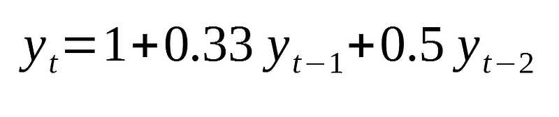
Since we are dealing with an autoregressive model of order 2, we need to define the coefficient at lag 0, 1 and 2.

Also, we will cancel the effect of a moving average process.

Finally, we will generate 10 000 data points.

In code:

ar2 = np.array([1, 0.33, 0.5])
ma = np.array([1])

simulated_AR2_data = ArmaProcess(ar2, ma).generate_sample(nsample=10000)

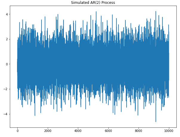
We can plot the time series:

plt.figure(figsize=[10, 7.5]); # Set dimensions for figure
plt.plot(simulated_AR2_data)
plt.title("Simulated AR(2) Process")
plt.show()

And you should get something similar to this:

Now, let’s take a look at the autocorrelation plot (correlogram):

plot_acf(simulated_AR2_data);

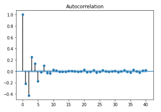
You can see that the coefficient is slowly decaying. This means that it is unlikely a moving average process and it suggests that the time series can probably be modelled with an autoregressive process (which makes sense since that what we are simulating).

To make sure that this is right, let’s plot the partial autocorrelation plot:

plot_pacf(simulated_AR2_data);

As you can see the coefficients are not significant after lag 2. Therefore, the partial autocorrelation plot is useful to determine the order of an AR(p) process.

You can also check the values of each coefficients by running:

pacf_coef_AR2 = pacf(simulated_AR2_data)
print(pacf_coef_AR2)

Now, in a real project setting, it can be easy to find the order of an AR(p) process, but we need to find a way to estimate the coefficients phi.

To do so, we use the Yule-Walker equation. This equations allows us to estimate the coefficients of an AR(p) model, given that we know the order.

rho, sigma = yule_walker(simulated_AR2_data, 2, method='mle')
print(f'rho: {-rho}')
print(f'sigma: {sigma}')

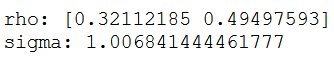
As you can see, the Yule-Walker equation did a decent job at estimating our coefficients and got very close to 0.33 and 0.5.

Simulation of an AR(3) process

Now, let’s simulate an AR(3) process. Specifically, we will simulate:

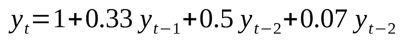
Similarly to what was previously done, let’s define our coefficients and generate 10 000 data points:

ar3 = np.array([1, 0.33, 0.5, 0.07])
ma = np.array([1])

simulated_AR3_data = ArmaProcess(ar3,ma).generate_sample(nsample=10000)

Then, we can visualize the time series:

plt.figure(figsize=[10, 7.5]); # Set dimensions for figure
plt.plot(simulated_AR3_data)
plt.title("Simulated AR(3) Process")
plt.show()

And you should see something similar to:

Now, looking at the PACF and ACF:

plot_pacf(simulated_AR3_data);
plot_acf(simulated_AR3_data);

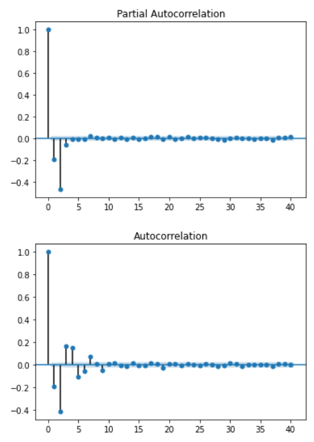
You see that the coefficients are not significant after lag 3 for the PACF function as expected.

Finally, let’s use the Yule-Walker equation to estimate the coefficients:

rho, sigma = yule_walker(simulated_AR3_data, 3, method='mle')
print(f'rho: {-rho}')
print(f'sigma: {sigma}')

Again, the estimations are fairly close to the actual values.

Project — Forecasting the quarterly EPS for Johnson&Johnson

Now, let’s apply our knowledge of autoregressive processes in a project setting.

The objective is to model the quarterly earnings per share (EPS) of the company Johnson&Johnson between 1960 and 1980.

First, let’s read the dataset:

import pandas as pd

data = pd.read_csv('jj.csv')
data.head()

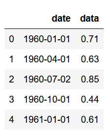
Now, the first five rows are not very useful for us. Let’s plot the entire dataset to get a better visual representation.

plt.figure(figsize=[15, 7.5]); # Set dimensions for figure
plt.scatter(data['date'], data['data'])
plt.title('Quaterly EPS for Johnson & Johnson')
plt.ylabel('EPS per share ($)')
plt.xlabel('Date')
plt.xticks(rotation=90)
plt.grid(True)
plt.show()

Awesome! Now we can the there is clear upwards trend in the data. While this may be a good sign for the company, it is not good in terms of time series modelling, since it means that the time series is not stationary.

As aforementioned, the AR(p) process works only for stationary series.

Therefore, we must apply some transformations to our data to make it stationary.

In this case, will take the log difference. This is equivalent to taking the log of each value, and subtracting the previous value.

# Take the log difference to make data stationary

data['data'] = np.log(data['data'])
data['data'] = data['data'].diff()
data = data.drop(data.index[0])
data.head()

Plotting the transformed time series:

plt.figure(figsize=[15, 7.5]); # Set dimensions for figure
plt.plot(data['data'])
plt.title("Log Difference of Quaterly EPS for Johnson & Johnson")
plt.show()

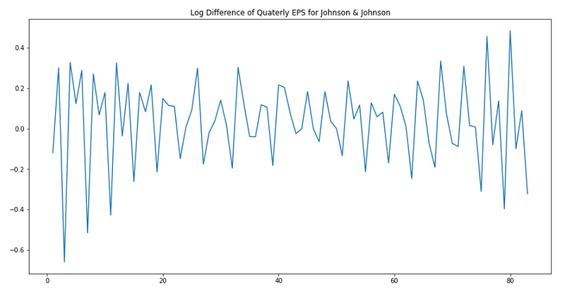
Now, it seems that we removed the trend. However, we have to be sure that our series is stationary before modelling with an AR(p) process.

We will thus use the augmented Dicker-Fuller test. This will give us the statistical confidence that our time series is indeed stationary.

ad_fuller_result = adfuller(data['data'])
print(f'ADF Statistic: {ad_fuller_result[0]}')
print(f'p-value: {ad_fuller_result[1]}')

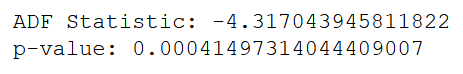
Since we get a large negative ADF statistic and p-value smaller than 0.05, we can reject the null hypothesis and say that our time series is stationary.

Now, let’s find the order of the process by plotting the PACF:

plot_pacf(data['data']);
plot_acf(data['data']);

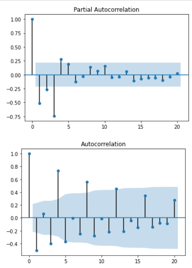
As you can see, after lag 4, the PACF coefficients are not significant anymore. Therefore, we will assume an autoregressive process of order 4.

Now, we will use this information to estimate the coefficients using the Yule-Walker equation:

# Try a AR(4) model
rho, sigma = yule_walker(data['data'], 4)
print(f'rho: {-rho}')
print(f'sigma: {sigma}')

Therefore, the function is approximated as:

Note that this equation models the transformed series.

Conclusion

Congratulations! You now understand what an autoregressive model is, how to recognize an autoregressive process, how to determine its order, and how to use it to model a real-life time series.

Sharpen your time series analysis skills with my free time series cheat sheet!

Cheers 🍺

Support me

Enjoying my work? Show your support with Buy me a coffee, a simple way for you to encourage me, and I get to enjoy a cup of coffee! If you feel like it, just click the button below 👇