Time-LLM: Reprogram an LLM for Time Series Forecasting

It is not the first time that researchers try to apply natural language processing (NLP) techniques to the field of time series.

For example, the Transformer architecture was a significant milestone in NLP, but its performance in time series forecasting remained average, until PatchTST was proposed.

As you know, large language models (LLMs) are being actively developed and have demonstrated impressive generalization and reasoning capabilities in NLP.

Thus, it is worth exploring the idea of repurposing an LLM for time series forecasting, such that we can benefit from the capabilities of those large pre-trained models. 

To that end, Time-LLM was proposed. In the original paper, the researchers propose a framework to reprogram an existing LLM to perform time series forecasting.

In this article, we explore the architecture of Time-LLM and how it can effectively allow an LLM to predict time series data. Then, we implement the model and apply it in a small forecasting project.

For more details, make sure to read the original paper.

Learn the latest time series analysis techniques with my free time series cheat sheet in Python! Get the implementation of statistical and deep learning techniques, all in Python and TensorFlow!

Let’s get started!

Explore Time-LLM

Time-LLM is to be considered more as a framework than an actual model with a specific architecture.

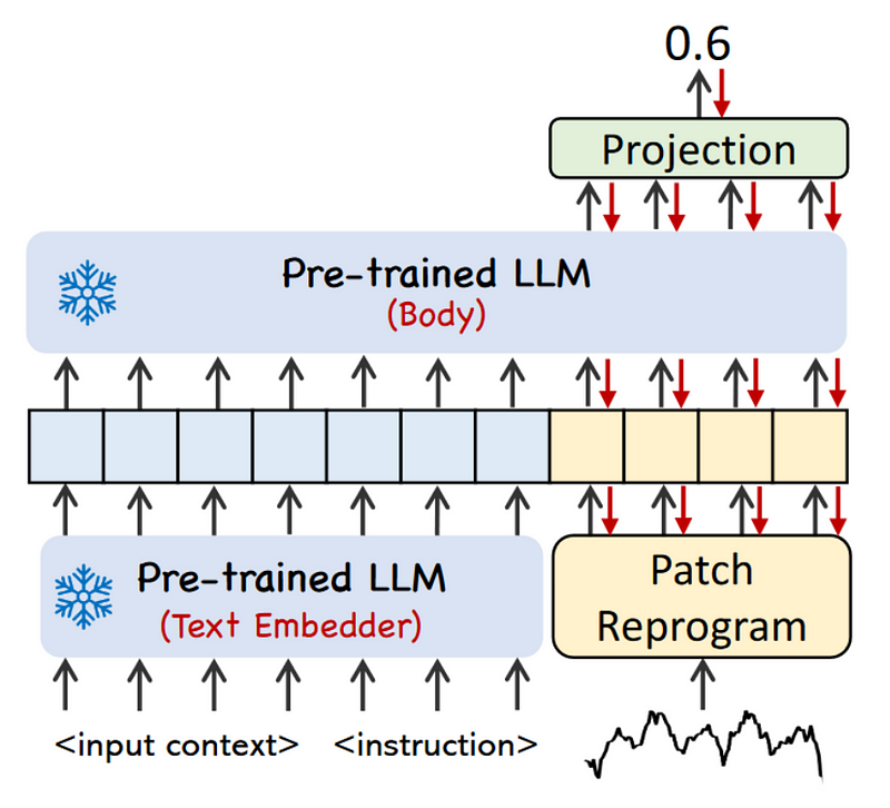
The general structure of Time-LLM is shown below.

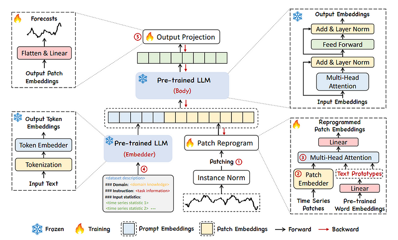
The entire idea behind Time-LLM is to reprogram an embedding-visible language foundation model, like LLaMA or GPT-2.

Note that this is different from fine-tuning the LLM. Instead, we teach the LLM to take an input sequence of time steps and output forecasts over a certain horizon. This means that the LLM itself stays unchanged.

At a high level, Time-LLM starts by tokenizing the input time series sequence with a customized patch embedding layer. These patches are then sent through a reprogramming layer that essentially translate the forecasting task into a language task. Note that we can also pass a prompt prefix to augment the model’s reasoning ability. Finally, the output patches go through the projection layer to ultimately get forecasts.

There is a lot to dissect here, so let’s explore each step in more detail.

Input patching

The first step is to patch the input series, just like in PatchTST.

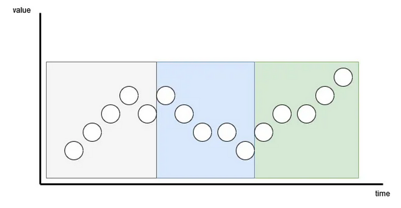
With patching, the goal is to preserve the local semantic information by looking at groups of time steps instead of looking at a single time step.

It also has the added benefit of greatly reducing the number of token being fed to the reprogramming layer. Here, each patch becomes an input token so it reduces the number of tokens from L to approximately L/S, where L is the length of the input sequence, and S is the stride length.

Once patching is done, the input sequence is sent to the reprogramming layer.

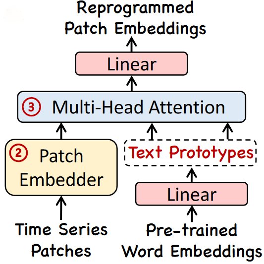
Reprogramming layer

In Time-LLM, the language model stays intact. 

Now, a language model can perform many NLP tasks, like sentiment analysis, summarization and text generation, but time series forecasting.

This is where the reprogramming layer comes in. It essentially maps the input time series into a language task, allowing us to leverage the capabilities of the language model.

To do so, it uses a restricted vocabulary to describe each input patch, as shown below.

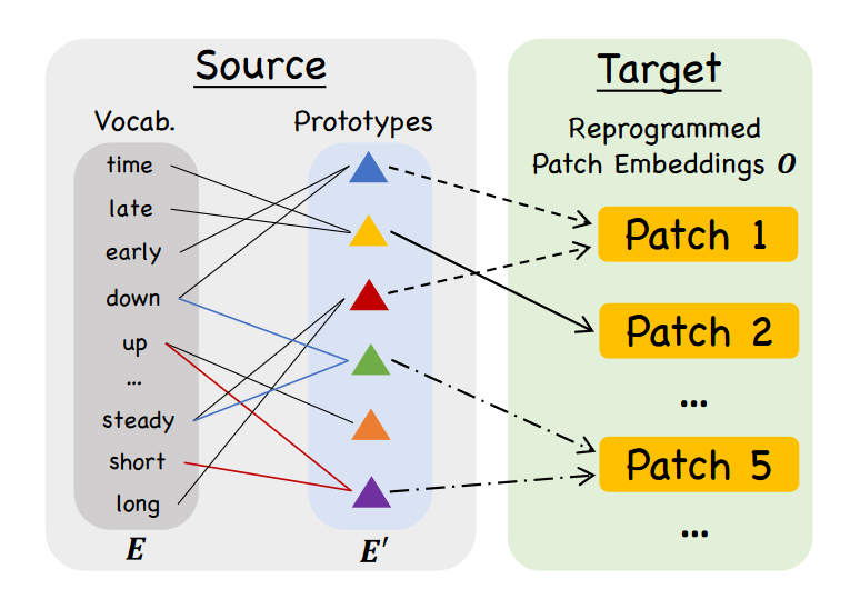
In the figure above, we can see how each time series patch gets described. For example, one patch could be translated to “short up then steadily down”. That way, we effectively encode the behavior of the time series as a natural language input, which is what the LLM expects. 

Once this is done, the translated patches are sent to a multi-head attention mechanism and a linear projection is done to align the dimension of the reprogrammed patches to the dimension of the LLM backbone.

Note that the reprogramming layer is a trained layer. We can decide to train it for a specific dataset, or pre-train it and use Time-LLM as a zero-shot forecaster.

Now, before the translated patches are actually sent to the LLM, it is possible to augment the input using a prompt prefix.

Augment the input with Prompt-as-Prefix

To activate the LLM’s capabilities, we use a prompt, which a natural language input specifying the task for the LLM.

Now, even though we are passing patches of time series translated to natural language, it still represents a challenge for the LLM to make predictions. 

Therefore, the researchers propose to use a prompt prefix to complement patch reprogramming. 

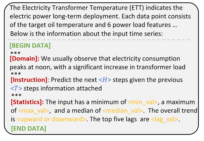
In the figure above, we see an example of prompt prefix on the benchmark dataset ETT.

The prompt contains three distinct parts:

1. General context of the dataset
2. Task instructions
3. Input statistics

The first component is entirely defined by the user. This is where we can specify information on the dataset, explain its context and write out the observations.

Then, the task instructions are set programmatically given the horizon of the forecast and the input size of the series.

Finally, the input statistics are also computed automatically given the input series. Note that the top five lags are calculated using a fast Fourier transform. In short, it transforms the input series into a function of amplitude and frequency, and the frequencies with the highest amplitudes are considered to be more important. 

So, at this point, we have a prompt prefix containing context and instructions for the LLM, as well as reprogrammed patches of the series being fed to the LLM, as shown below.

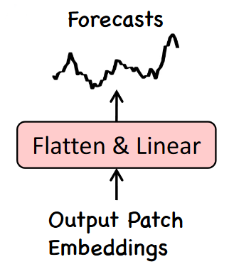
The final step in the framework is to send the output patch embeddings through a linear projection layer to get the final predictions.

Output projection

Once the prompt prefix and reprogrammed patches are sent to the LLM, it outputs patch embeddings.

This output must then be flattened and projected linearly to derive the final forecasts, as shown below.

To summarize the flow through Time-LLM:

• An input series is first patched and reprogrammed as a language task. 
• We append to it a prompt prefix specifying the context of the data, the instructions for the LLM, and input statistics. 
• The combined input is sent to the LLM.
• The output embeddings are flattened and projected to generate predictions.

Now that we understand the inner workings of Time-LLM, let’s apply it in s small experiment using Python.

Forecasting with Time-LLM

In this little experiment, we apply Time-LLM for time series forecasting and compare its performance to other models like N-HiTS and a simple multilayer perceptron (MLP).

Before getting started, I must mention the following:

1. I will be extending the library neuralforecast with Time-LLM, as I think that the original codebase of Time-LLM is hard to use.
2. I am not the best prompt engineer and since Time-LLM relies on an LLM, you might be able to get better results than me with a better context prompt.
3. The original paper reports performance obtained using LLaMA. Now, the license of LLaMA is restrictive, and it can only be used for research purposes. For that reason, I will use GPT-2. Of course, using other LLMs is likely going to give different results.
4. I have limited time and compute power. I trained Time-LLM for 100 epochs on a single GPU. If you have more time and a better GPU, you can train the model for longer and potentially get better results.

The code for this experiment is available on GitHub.

Let’s get started!

Extend neuralforecast with Time-LLM

For this experiment, I will implement Time-LLM in the library neuralforecast to make it easier and more flexible to use than the paper’s implementation.

Following the contribution guidelines of neuralforecast, we start by creating a TimeLLMclass that inherits from BaseWindowswhich takes care of parsing batches of the input time series.

Then, in the __init__ function, we specify the parameters associated with Time-LLM, followed by the inherited parameters of BaseWindows.

class TimeLLM(BaseWindows):
    def __init__(self,
                 h,
                 input_size,
                 patch_len: int = 16,
                 stride: int = 8,
                 d_ff: int = 128,
                 top_k: int = 5,
                 d_llm: int = 768,
                 d_model: int = 32,
                 n_heads: int = 8,
                 enc_in: int = 7,
                 dec_in: int  = 7,
                 llm = None,
                 llm_config = None,
                 llm_tokenizer = None,
                 llm_num_hidden_layers = 32,
                 llm_output_attention: bool = True,
                 llm_output_hidden_states: bool = True,
                 prompt_prefix: str = None,
                 dropout: float = 0.1,
                # Inherited parameters of BaseWindows

In the code block above, we see that we have parameters for patching, as well as for the LLM that we wish to use. 

Unlike the original implementation which uses LLaMA, this implementation allows the user to choose any LLM of their choice using the transformers library.

Then, we reuse the same logic of the original implementation, but modify the forwardmethod to follow the guidelines of neuralforecast.

def forward(self, windows_batch):
    insample_y = windows_batch['insample_y']
    
    x = insample_y.unsqueeze(-1)
    
    y_pred = self.forecast(x)
    y_pred = y_pred[:, -self.h:, :]
    y_pred = self.loss.domain_map(y_pred)
    
    return y_pred

In the code block above, we use windows_batch to access an input batch and run it through Time-LLM. Then, we use self.loss.domain_map(y_pred) to map the output to the domain and shape of the chosen loss function. This is necessary for the model to actually train.

For the fully detailed implementation, you can look here (it is still being actively developed, so changes might occur by the time you read this).

Then, we simply add the model to the appropriate init file, and we can run pip install . to have access to the new model.

Just like that, we can now use Time-LLM in neuralforecast.

Predicting with Time-LLM

We are now ready to forecasting with Time-LLM. Here, we use the simple air passenger’s dataset. 

First, let’s import the required libraries.

import time
import numpy as np
import pandas as pd
import pytorch_lightning as pl
import matplotlib.pyplot as plt

from neuralforecast import NeuralForecast
from neuralforecast.models import TimeLLM
from neuralforecast.losses.pytorch import MAE
from neuralforecast.tsdataset import TimeSeriesDataset
from neuralforecast.utils import AirPassengers, AirPassengersPanel, AirPassengersStatic, augment_calendar_df

from transformers import GPT2Config, GPT2Model, GPT2Tokenizer

Then, we load the dataset, which is conveniently included in neuralforecast.

AirPassengersPanel, calendar_cols = augment_calendar_df(df=AirPassengersPanel, freq='M')

Y_train_df = AirPassengersPanel[AirPassengersPanel.ds<AirPassengersPanel['ds'].values[-12]]
Y_test_df = AirPassengersPanel[AirPassengersPanel.ds>=AirPassengersPanel['ds'].values[-12]].reset_index(drop=True)

Then, we need to choose an LLM. For this experiment, let’s go with GPT-2. We can load the model, its configuration and tokenizer from transformers.

gpt2_config = GPT2Config.from_pretrained('openai-community/gpt2')
gpt2 = GPT2Model.from_pretrained('openai-community/gpt2',config=gpt2_config)
gpt2_tokenizer = GPT2Tokenizer.from_pretrained('openai-community/gpt2')

Then, we can define a prompt to explain the context of the data. Here, I used the following prompt:

prompt_prefix = "The dataset contains data on monthly air passengers. There is a yearly seasonality"

Then, we can initialize the model using:

timellm = TimeLLM(h=12,
                 input_size=36,
                 llm=gpt2,
                 llm_config=gpt2_config,
                 llm_tokenizer=gpt2_tokenizer,
                 prompt_prefix=prompt_prefix,
                 max_steps=100,
                 batch_size=24,
                 windows_batch_size=24)

Note that I am only training the reprogramming layer for 100 epochs and with a relatively small batch size. If you have more computing power, it might be better to increase max_steps, batch_size, and windows_batch_size.

Then, we can train the model and get predictions.

nf = NeuralForecast(
    models=[timellm],
    freq='M'
)

nf.fit(df=Y_train_df, val_size=12)
forecasts = nf.predict(futr_df=Y_test_df)

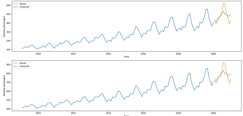
In the figure above, we can see that we successfully obtain time series forecasts while using the GPT-2 model, which I think is exciting and amazing!

However, the predictions are not great. The peak is totally missed, and even the trend does not seem to be considered in this case.

Now, there are many factors that could improve the performance, like:

• Training the model for longer. I trained for 100 epochs, but the paper uses 1000 epochs.
• Change LLM. I used GPT-2, but LLaMA, which was used in the paper, is much better. Maybe that using a Mistral model or Gemma would help.
• Better prompt. My prompt is very minimal, and perphas we can better engineer it.

Keep in mind that the goal is to show you how to use Time-LLM for your own use case, and not get state-of-the-art results. While my resources were restricted, we can still use any LLM we want to forecast any time series dataset, and that is the real advantage of this implementation.

Still, for the sake of comleteness, let’s compare Time-LLM to other models.

Forecasting with N-BEATS and MLP

My run with Time-LLM did not generate the best predictions, but let’s still use other models to see how they perform.

Specifically, we use N-BEATS and a simple MLP model. Here too, I will train for only 100 epochs, but feel free to train for longer.

nbeats = NBEATS(h=12, input_size=36, max_steps=100)
mlp = MLP(h=12, input_size=36, max_steps=100)

nf = NeuralForecast(models=[nbeats, mlp], freq='M')

nf.fit(df=Y_train_df, val_size=12)
forecasts = nf.predict(futr_df=Y_test_df)

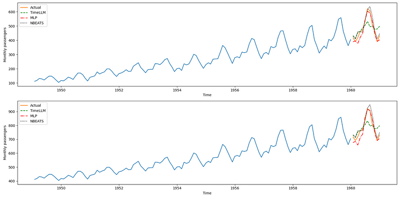
Unsurprisingly, N-BEATS and the MLP perform much better than Time-LLM, but again, keep in mind that my run of Time-LLM is far from being optimized.

Still, let’s evaluate the performance using the mean absolute error (MAE).

from neuralforecast.losses.numpy import mae

mae_timellm = mae(Y_test_df['y'], Y_test_df['TimeLLM'])
mae_nbeats = mae(Y_test_df['y'], Y_test_df['NBEATS'])
mae_mlp = mae(Y_test_df['y'], Y_test_df['MLP'])

data = {'Time-LLM': [mae_timellm], 
       'N-BEATS': [mae_nbeats],
       'MLP': [mae_mlp]}

metrics_df = pd.DataFrame(data=data)
metrics_df.index = ['mae']

metrics_df.style.highlight_min(color='lightgreen', axis=1)

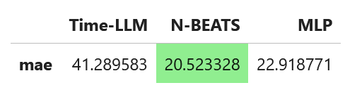
In this case, N-BEATS achieves the best performance as it has the lowest MAE.

Again, the results for Time-LLM might be underwhelming, but there are many ways to improve upon my experiment since I had limited resources as aforementioned.

Also, this was a very simple experiment on a toy dataset. The goal is to show how to use Time-LLM in any situation, rather than benchmark the model against other methods.

My opinion on Time-LLM

LLMs represent a giant leap forward in the field of NLP, and with their application in computer vision too, it only make sense to see them being applied for time series forecasting.

Still, would I use Time-LLM in a forecasting project?

Probably not. 

The reality is that Time-LLM requires a lot of computing power and memory. After all, we are working with an LLM.

In fact, when reproducing the results from the paper using their script, training the model on a single dataset for 1000 epochs takes approximately 19 hours using a GPU!

Plus, LLMs take a lot of memory space, with billions of parameter usually weighing a few gigabytes for the very large models. In comparison, we can train lightweight deep learning models in a few minutes and get very good forecasts.

For those reasons, I think that the tradeoff between a possible increase in forecasts accuracy and the computing power and memory storage required to run such model is not worth it.

Still, it is exciting to see that time series forecasting can now benefit from the advances in LLMs, which is an actively researched field. If LLMs get better and lighter, maybe Time-LLM will become an interesting option.

Conclusion

Time-LLM is a framework that allows any embedding-visible LLM to be used for time series forecasting.

It first patches the input series to tokenize it and reprogram it as a language task, by traning a reprogramming layer.

It also adds a prompt prefix to provide the LLM with the context of the dataset, the forecasting task, and some input statistics.

Then, by keeping the LLM model intact, we can pass the reprogrammed patches and prompt to the LLM and obtain forecasts.

As always, I think that each problem requires its unique solution. Make sure to test Time-LLM against other methods.

Thanks for reading! I hope that you enjoyed it and that you learned something new!

Cheers 🍻

Learn the latest time series analysis techniques with my free time series cheat sheet in Python! Get the implementation of statistical and deep learning techniques, all in Python and TensorFlow!

Support me

Enjoying my work? Show your support with Buy me a coffee, a simple way for you to encourage me, and I get to enjoy a cup of coffee! If you feel like it, just click the button below 👇

References

Time-LLM: Time Series Forecasting by Reprogramming Large Language Models by M. Jin, S. Wang, L. Ma, Z. Chu, J. Zhang, X. Shi, P. Chen, Y. Liang, Y. Li, S. Pan, Q. Wen

Original repository of Time-LLM — GitHub