Theta Model for Time Series Forecasting

When it comes to time series forecasting, we often turn our attention to models in the SARIMAX family or exponential smoothing. However, there is one forecasting technique that is rarely mentioned: the Theta model.

Despite its simplicity, the Theta model can generate accurate predictions. It performed so well during the M-3 competition, the largest academic time series forecasting competition, that it became a benchmark in the following years.

In this article, we first explore the inner workings of the model from a theoretical point of view. Then, we apply the Theta model in a forecasting exercise and compare its performance to SARIMA model and an exponential smoothing model. Of course, all the code is in Python.

Let’s get started!

Learn the latest time series analysis techniques with my free time series cheat sheet in Python! Get the implementation of statistical and deep learning techniques, all in Python and TensorFlow!

How the Theta model works

The Theta model basically relies on decomposition. We know that time series can be decomposed into three components: a trend component, a seasonal component and residuals. 

Thus, it is a reasonable approach to decompose a series into each of its components, forecast each component into the future, and combine the predictions of each component to create your final predictions.

Unfortunately, this does not work in practice, especially because it is hard to isolate the residuals and forecast them.

So the Theta model is an evolution of this idea, but it relies in decomposing the series into a long-term component and a short-term component.

In formal terms, the Theta model is based on the concept of modifying the local curvature of the time series. This modification is managed by a parameter called theta (hence the name Theta model). This modification is applied on the second difference of the series, meaning that it is differenced twice.

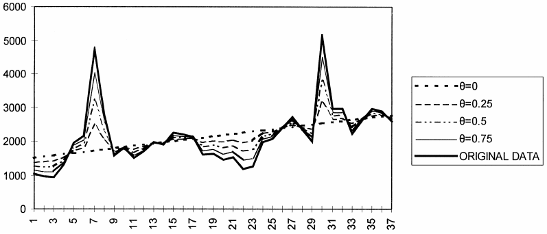
When theta is between 0 and 1, the series is “deflated”. That means that short-term fluctuations are smaller, and we emphasize on long-term effects. When theta reaches 0, the series is transformed into a linear regression line. This behaviour is shown in the figure below.

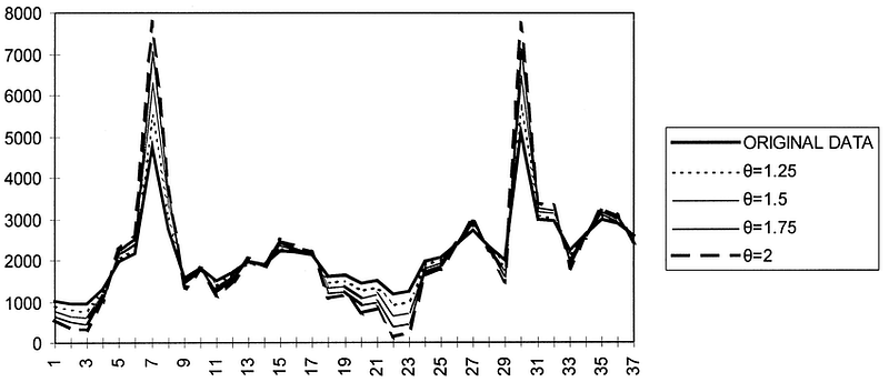
Alternatively, when theta is greater than 1, then the short-term fluctuations are magnified, and so we emphasize on the short-term effects. In that case, we also say that the series is “inflated”. This behaviour is shown in the figure below.

For each value of theta, we say the we create a “theta line”. In theory, we can generate as many theta line as we want, forecast each into the future, and combine them for a final prediction. 

In practice, we often use only two theta lines: one where theta is 0, and one where theta is 2. The first theta line (theta = 0) gives information about the trend of the series, while the second theta line (theta = 2) magnifies the short-term fluctuations. Then, we forecast each line, and combine the predictions.

What about seasonality?

The Theta model’s procedure is applied on non-seasonal data. However, it can still be used with seasonal data, as that seasonality can easily be removed and added back again at the end.

Thus, the implementation of the Theta model follows these steps:

1. Remove seasonality: a test for seasonality is performed. If seasonality is detected, it is removed by decomposition.
2. Decompose into two theta lines: we generate the two theta line; one where theta = 0, denoted as Z(0), and one where theta = 2 denoted as Z(2).
3. Extrapolation: we extrapolate both theta lines into the future. Z(0) is extrapolated using a linear regression, since it is a linear regression line itself. Z(2) is extrapolated using simple exponential smoothing.
4. Combination: we combine the extrapolation of both theta lines to obtain a single predicted line.
5. Add seasonality back: if seasonality was removed in the first step, we add it back at the end.

Now that we understand how the Theta model works, let’s apply it in a forecasting exercise!

Forecasting with the Theta model

For this exercise, we will forecast the CO2 concentration as recorded at Mauna Loa Observatory, from March 1958 to December 2001. The data was recorded every week.

At any point, feel free to consult the source code on GitHub.

The first step is of course to import the necessary libraries and load the data.

import numpy as np
import pandas as pd
import statsmodels.api as sm
import matplotlib.pyplot as plt

# Load the data
df = sm.datasets.co2.load_pandas().data
df.head()

We can then visualize our dataset. The result is shown in the figure below.

fig, ax = plt.subplots()

ax.plot(df['co2'])
ax.set_xlabel('Time')
ax.set_ylabel('CO2 concentration (ppmw)')

fig.autofmt_xdate()
plt.tight_layout()

Looking at the figure above, we notice three important elements:

1. Our series has a positive trend, as CO2 concentration is increasing over time.
2. Our series has a yearly seasonality, as CO2 is higher during the winter than in the summer.
3. We have some missing values at the beginning of the dataset.

So, let’s get rid of the missing values. Here, we simply interpolate the missing values using two known points.

df = df.interpolate()

This takes care of any missing values, and we are ready to move on to forecasting.

Forecasting

For this situation, we reserve the last two years of observations for the test set. Since we have weekly data, and there are 52 weeks in a year, this means that the last 104 points are for the test set, and the rest is for training.

train = df[:-104]
test = df[-104:]

Then, we must set a forecast horizon. Here, we set it to 52 weeks, or a year. This means that we want to build a model that can predict the next 52 weeks of CO2 concentration.

Since our test set has 104 weeks of data, we will perform rolling forecasts. This means that we train the model on the training set, predict the next 52 weeks, then retrain the model on an updated training set that includes another 52 weeks of data to forecast the next 52 weeks. 

It is fairly confusing to describe rolling forecasts in words, so here is a diagram to visualize the entire process.

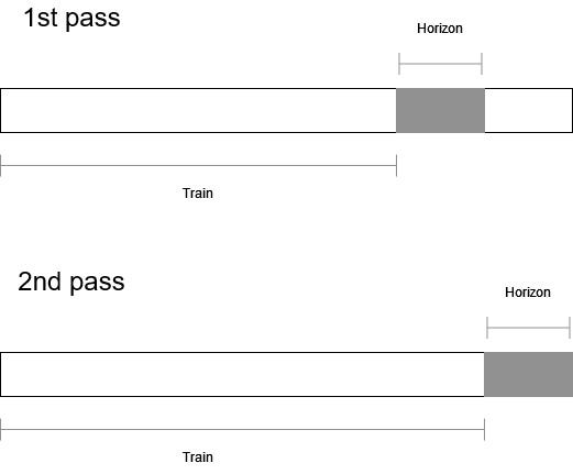
From the figure above, we can see that we forecast the entire test set of 104 weeks, but 52 weeks at a time. That way, we simulate the process of collecting new data and adding to the training set before making new predictions.

Before moving on, we also need to choose a baseline model. Here, since we have seasonal data, a reasonable baseline would be to simply forecast the last know season. Since we have a yearly seasonality, and 52 observations per year, this is equivalent to repeating the last 52 data points into the future.

With all that set, we can now build up our function to make rolling forecasts.

from statsmodels.tsa.forecasting.theta import ThetaModel

def rolling_forecast(df: pd.DataFrame, train_len: int, horizon: int, window: int, method: str) -> list:
    
    total_len = train_len + horizon
    end_idx = train_len

if method == 'last_season':
        pred_last_season = []
        
        for i in range(train_len, total_len, window):
            last_season = df[:i].iloc[-window:].values
            pred_last_season.extend(last_season)
            
        return pred_last_season
    
    elif method == 'theta':
        pred_theta = []
        
        for i in range(train_len, total_len, window):
            tm = ThetaModel(endog=df[:i], period=52)
            res = tm.fit()
            predictions = res.forecast(window)
            pred_theta.extend(predictions)
            
        print(res.summary()) #Optional

return pred_theta

Above, we see that our function needs a time series dataset, the initial length of the training set, the length of the test set and a window or a horizon.

The length of the training set and the test set is easily recovered from the split we made previously, and our window will be 52 weeks, as mentioned before.

TRAIN_LEN = len(train)
HORIZON = len(test)
WINDOW = 52

We are now ready to forecast our time series, using both the baseline model and the Theta model.

test = test.copy()

test.loc[:, 'pred_last_season'] = pred_last_season
test.loc[:, 'pred_theta'] = pred_theta

test.head()

Adding triple exponential smoothing

For the sake of comparison, let’s also apply triple exponential smoothing in this situation. That way, we can compare the performance of the Theta model to both the baseline and another relatively simple model.

To do so, we must update our rolling_forecast function to implement triple exponential smoothing.

from statsmodels.tsa.holtwinters import ExponentialSmoothing

def rolling_forecast(df: pd.DataFrame, train_len: int, horizon: int, window: int, method: str) -> list:
    
    total_len = train_len + horizon
    end_idx = train_len

if method == 'last_season':
        pred_last_season = []
        
        for i in range(train_len, total_len, window):
            last_season = df[:i].iloc[-window:].values
            pred_last_season.extend(last_season)
            
        return pred_last_season
    
    elif method == 'theta':
        pred_theta = []
        
        for i in range(train_len, total_len, window):
            tm = ThetaModel(endog=df[:i], period=52)
            res = tm.fit()
            predictions = res.forecast(window)
            pred_theta.extend(predictions)

return pred_theta
            
    elif method == 'tes':
        pred_tes = []
        
        for i in range(train_len, total_len, window):
            tes = ExponentialSmoothing(
                df[:i],
                trend='add',
                seasonal='add',
                seasonal_periods=52,
                initialization_method='estimated'
            ).fit()
            
            predictions = tes.forecast(window)
            pred_tes.extend(predictions)

return pred_tes

Then, we simply run it to add the predictions coming from triple exponential smoothing.

pred_tes = rolling_forecast(df, TRAIN_LEN, HORIZON, WINDOW, 'tes')

test.loc[:, 'pred_tes'] = pred_tes

test.head()

Evaluation

Now that we have predictions from the baseline, the Theta model, and triple exponential smoothing, let’s evaluate each and determine the champion model. 

Here, we use the mean absolute percentage error, or MAPE, to evaluate our models.

Before actually measuring the performance, let’s first visualize the predictions of our models against the actual values. The result is shown in the figure below.

fig, ax = plt.subplots()

ax.plot(df['co2'])
ax.plot(test['co2'], 'b-', label='actual')
ax.plot(test['pred_last_season'], 'r:', label='baseline')
ax.plot(test['pred_theta'], 'g-.', label='Theta')
ax.plot(test['pred_tes'], 'k--', label='TES')

ax.set_xlabel('Time')
ax.set_ylabel('CO2 concentration (ppmv)')
ax.axvspan('2000-01-08', '2001-12-29', color='#808080', alpha=0.2)

ax.legend(loc='best')

ax.set_xlim('1998-03-07', '2001-12-29')

fig.autofmt_xdate()
plt.tight_layout()

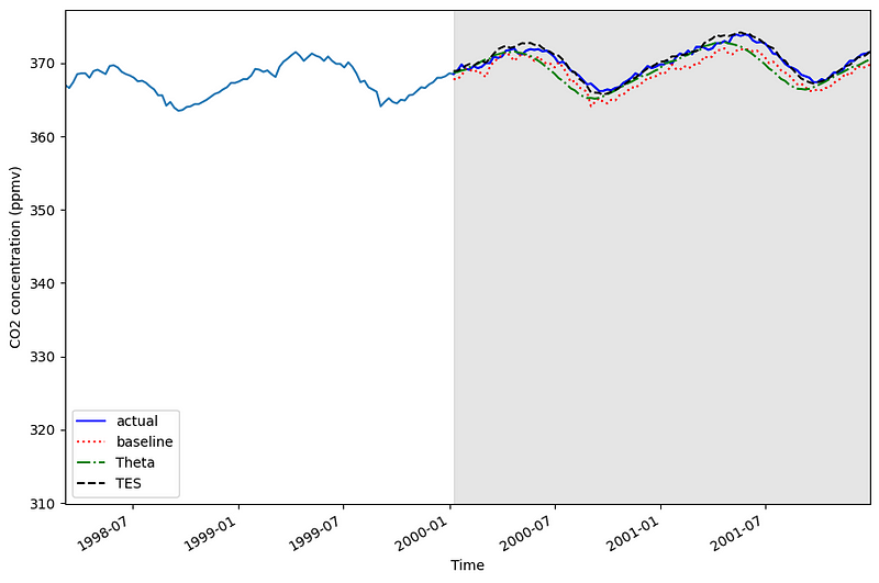
Looking at the figure above, we can see that the predictions from the baseline are the farthest from the actual values. We also see that line from triple exponential smoothing (black dashed line) seems to be the closest to the actual values.

Let’s verify that by actually computing the MAPE.

def mape(y_true, y_pred):
    return round(np.mean(np.abs((y_true - y_pred) / y_true)) * 100, 2)

mape_baseline = mape(test['co2'], test['pred_last_season'])
mape_theta = mape(test['co2'], test['pred_theta'])
mape_tes = mape(test['co2'], test['pred_tes'])

Note that at the time of writing this article, MAPE is still not implemented in the stable version of scikit-learn, but it is coming soon!

Finally, let’s visualize the MAPE of each model in a bar chart.

fig, ax = plt.subplots()

x = ['Baseline', 'Theta', 'TES']
y = [mape_baseline, mape_theta, mape_tes]

ax.bar(x, y, width=0.4)
ax.set_xlabel('Exponential smoothing models')
ax.set_ylabel('MAPE (%)')
ax.set_ylim(0, 1)

for index, value in enumerate(y):
    plt.text(x=index, y=value + 0.05, s=str(value), ha='center')
    
plt.tight_layout()

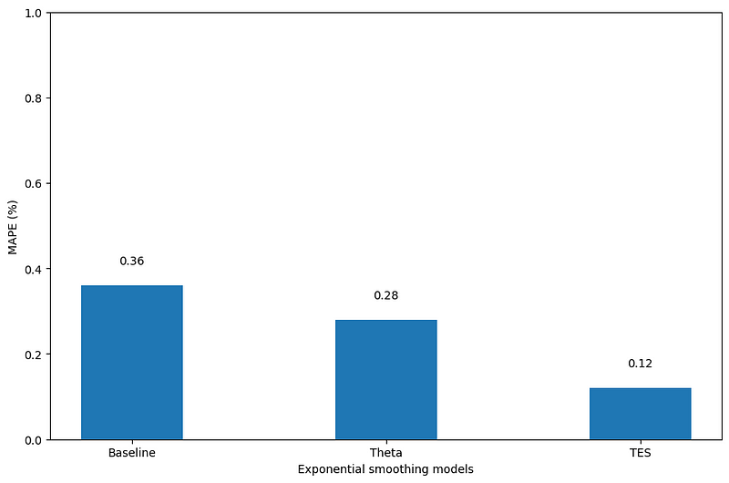
Looking at the figure above, we can see that our champion model is triple exponential smoothing as it achieves a MAPE of 0.12%. 

As for the Theta model, it outperforms the baseline, but it is worse than triple exponential smoothing.

Conclusion

Although the Theta model was not the champion model in this particular situation, it remains a great forecasting method to keep in your toolbox.

Its decomposition approach makes it a flexible and fast method for forecasting time series. At the very least, it can serve as a solid benchmark to compare other more complex models.

That’s it for this article! Congrats on making it to the end and I hope you enjoyed it and learned something new!

Make sure to download my free time series forecasting cheat sheet in Python, covering both statistical and deep learning models!

Cheers 🍺

Support me

Enjoying my work? Show your support with Buy me a coffee, a simple way for you to encourage me, and I get to enjoy a cup of coffee! If you feel like it, just click the button below 👇

References

Grzegorz Dudek — Short-term load forecasting using Theta method

Rob J. Hyndman, Baki Billah — Unmasking the Theta method

V. Assimakopoulos, K. Nikolopoulos — The theta model: a decomposition approach to forecasting

K. Nikolopoulos, V. Assimakopoulos, N. Bougioukos, A. Litsa — The Theta Model: An Essential Forecasting Tool for Supply Chain Planning