PatchTST: A Breakthrough in Time Series Forecasting

Transformer-based models have been successfully applied in many fields like natural language processing (think BERT or GPT models) and computer vision to name a few.

However, when it comes to time series, state-of-the-art results have mostly been achieved by MLP models (multilayer perceptron) such as N-BEATS and N-HiTS. A recent paper even shows that simple linear models outperform complex transformer-based forecasting models on many benchmark datasets (see Zheng et al., 2022).

Still, a new transformer-based model has been proposed that achieves state-of-the-art results for long-term forecasting tasks: PatchTST. 

PatchTST stands for patch time series transformer, and it was first proposed in March 2023 by Nie, Nguyen et al in their paper: A Time Series is Worth 64 Words: Long-Term Forecasting with Transformers. Their proposed method achieved state-of-the-art results when compared to other transformer-based models.

In this article, we first explore the inner workings of PatchTST, using intuition and no equations. Then, we apply the model in a forecasting project and compare its performance to MLP models, like N-BEATS and N-HiTS, and assess its performance.

Of course, for more details about PatchTST, make sure to refer to the original paper.

Learn the latest time series analysis techniques with my free time series cheat sheet in Python! Get the implementation of statistical and deep learning techniques, all in Python and TensorFlow!

Let’s get started!

Exploring PatchTST

As mentioned, PatchTST stands for patch time series transformer. 

As the name suggests, it makes use of patching and of the transformer architecture. It also includes channel-independence to treat multivariate time series. The general architecture is shown below.

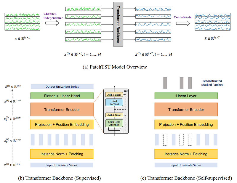
There is a lot of information to gather from the figure above. Here, the key elements are that PatchTST uses channel-independence to forecast multivariate time series. Then, in its transformer backbone, the model uses patching, which are illustrated by the small vertical rectangles. Also, the model comes in two versions: supervised and self-supervised.

Let’s explore in more detail the architecture and inner workings of PatchTST.

Channel-independence

Here, a multivariate time series is considered as a multi-channel signal. Each time series is basically a channel containing a signal. 

In the figure above, we see how a multivariate time series is separated into individual series, and each is fed to the Transformer backbone as an input token. Then, predictions are made for each series and the results are concatenated for the final predictions.

Patching

Most work on Transformer-based forecasting models focused on building new mechanisms to simplify the original attention mechanism. However, they still relied on point-wise attention, which is not ideal when it comes to time series.

In time series forecasting, we want to extract relationships between past time steps and future time steps to make predictions. With point-wise attention, we are trying to retrieve information from a single time step, without looking at what surrounds that point. In other words, we isolate a time step, and do not look at points before or after.

This is like trying to understand the meaning of a word without looking at the words around it in a sentence.

Therefore, PatchTST makes use of patching to extract local semantic information in time series.

How patching works

Each input series is divided into patches, which are simply shorter series coming from the original one.

Here, the patch can be overlapping or non-overlapping. The number of patches depends on the length of the patch P and the stride S. Here, the stride is like in convolution, it is simply how many timesteps separate the beginning of consecutive patches.

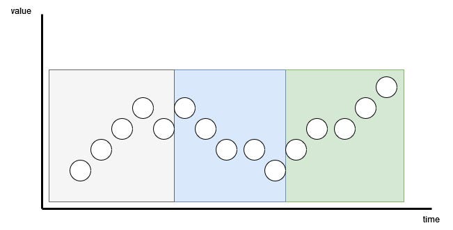
In the figure above, we can visualize the result of patching. Here, we have a sequence length (L) of 15 time steps, with a patch length (P) of 5 and a stride (S) of 5. The result is the series being separated into 3 patches. 

Advantages of patching

With patching, the model can extract local semantic meaning by looking at groups of time steps, instead of looking at a single time step.

It also has the added benefit of greatly reducing the number of token being fed to the transformer encoder. Here, each patch becomes an input token to be input to the Transformer. That way, we can reduce the number of token from L to approximately L/S.

That way, we greatly reduce the space and time complexity of the model. This in turn means that we can feed the model a longer input sequence to extract meaningful temporal relationships. 

Therefore, with patching, the model is faster, lighter, and can treat a longer input sequence, meaning that it can potentially learn more about the series and make better forecasts.

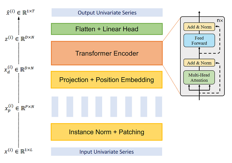
Transformer encoder

Once the series is patched, it is then fed to the transformer encoder. This is the classical transformer architecture. Nothing was modified.

Then, the output is fed to linear layer, and predictions are made.

Improving PatchTST with representation learning

The authors of the paper suggested another improvement to the model by using representation learning.

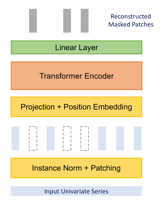
From the figure above, we can see that PatchTST can use self-supervised representation learning to capture abstract representations of the data. This can lead to potential improvements in forecasting performance.

Here, the process is fairly simple, as random patches will be masked, meaning that they will be set to 0. This is shown, in the figure above, by the blank vertical rectangles. Then, the model is trained to recreate the original patches, which is what is output at the top of the figure, as the grey vertical rectangles.

Now that we have a good understanding of how PatchTST works, let’s test it against other models and see how it performs.

Forecasting with PatchTST

In the paper, PatchTST is compared with other Transformer-based models. However, recent MLP-based models have been published, like N-BEATS and N-HiTS, and have also demonstrated state-of-the-art performance on long horizon forecasting tasks.

The complete source code for this section is available on GitHub.

Here, let’s apply PatchTST, along with N-BEATS and N-HiTS and evaluate its performance against these two MLP-based models.

For this exercise, we use the Exchange dataset, which is a common benchmark dataset for long-term forecasting in research. The dataset contains daily exchange rates of eight countries relative to the US dollar, from 1990 to 2016. The dataset is made available through the MIT License.

Initial setup

Let’s start by importing the required libraries. Here, we will work with neuralforecast, as they have an out-of-the-box implementation of PatchTST. For the dataset, we use the datasetsforecast library, which includes all popular datasets for evaluating forecasting algorithms.

import torch
import numpy as np
import pandas as pd
import matplotlib.pyplot as plt

from neuralforecast.core import NeuralForecast
from neuralforecast.models import NHITS, NBEATS, PatchTST

from neuralforecast.losses.pytorch import MAE
from neuralforecast.losses.numpy import mae, mse

from datasetsforecast.long_horizon import LongHorizon

If you have CUDA installed, then neuralforecast will automatically leverage your GPU to train the models. On my end, I do not have it installed, which is why I am not doing extensive hyperparameter tuning, or training on very large datasets.

Once that is done, let’s download the Exchange dataset.

Y_df, X_df, S_df = LongHorizon.load(directory="./data", group="Exchange")

Here, we see that we get three DataFrames. The first one contains the daily exchange rates for each country. The second one contains exogenous time series. The third one, contains static exogenous variables (like day, month, year, hour, or any future information that we know).

For this exercise, we only work with Y_df.

Then, let’s make sure that the dates have the right type.

Y_df['ds'] = pd.to_datetime(Y_df['ds'])

Y_df.head()

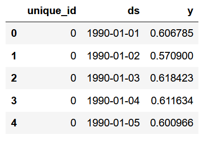
In the figure above, we see that we have three columns. The first column is a unique identifier and it is necessary to have an id column when working with neuralforecast. Then, the ds column has the date, and the y column has the exchange rate. 

Y_df['unique_id'].value_counts()

From the picture above, we can see that each unique id corresponds to a country, and that we have 7588 observations per country.

Now, we define the sizes of our validation and test sets. Here, I chose 760 time steps for validation, and 1517 for the test set, as specified by the datasets library.

val_size = 760
test_size = 1517

print(n_time, val_size, test_size)

Then, let’s plot one of the series, to see what we are working with. Here, I decided to plot the series for the first country (unique_id = 0), but feel free to plot another series.

u_id = '0'

x_plot = pd.to_datetime(Y_df[Y_df.unique_id==u_id].ds)
y_plot = Y_df[Y_df.unique_id==u_id].y.values

x_plot

x_val = x_plot[n_time - val_size - test_size]
x_test = x_plot[n_time - test_size]

fig, ax = plt.subplots(figsize=(12,8))
ax.plot(x_plot, y_plot)
ax.set_xlabel('Date')
ax.set_ylabel('Exhange rate')
ax.axvline(x_val, color='black', linestyle='--')
ax.axvline(x_test, color='black', linestyle='--')

plt.text(x_val, -2, 'Validation', fontsize=12)
plt.text(x_test,-2, 'Test', fontsize=12)

plt.tight_layout()

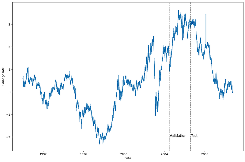
From the figure above, we see that we have fairly noisy data with no clear seasonality.

Modelling

Having explored the data, let’s get started on modelling with neuralforecast.

First, we need to set the horizon. In this case, I use 96 time steps, as this horizon is also used in the PatchTST paper.

Then, to have a fair evaluation of each model, I decided to set the input size to twice the horizon (so 192 time steps), and set the maximum number of epochs to 50. All other hyperparameters are kept to their default values.

horizon = 96

models = [NHITS(h=horizon,
               input_size=2*horizon,
               max_steps=50),
         NBEATS(h=horizon,
               input_size=2*horizon,
               max_steps=50),
         PatchTST(h=horizon,
                 input_size=2*horizon,
                 max_steps=50)]

Then, we initialize the NeuralForecastobject, by specifying the models we want to use and the frequency of the forecast, which in this is case is daily.

nf = NeuralForecast(models=models, freq='D')

We are now ready to make predictions.

Forecasting

To generate predictions, we use the cross_validation method to make use of the validation and test sets. It will return a DataFrame with predictions from all models and the associated true value.

preds_df = nf.cross_validation(df=Y_df, val_size=val_size, test_size=test_size, n_windows=None)

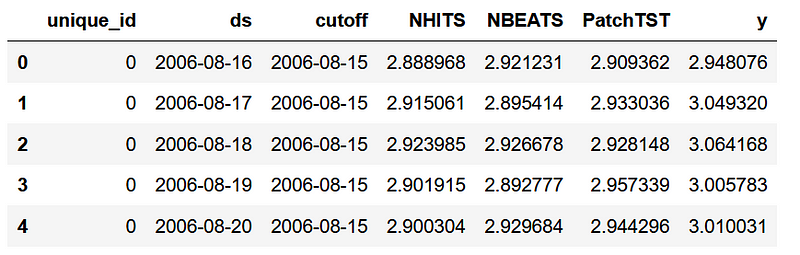
As you can see, for each id, we have the predictions from each model as well as the true value in the y column.

Now, to evaluate the models, we have to reshape the arrays of actual and predicted values to have the shape (number of series, number of windows, forecast horizon).

y_true = preds_df['y'].values
y_pred_nhits = preds_df['NHITS'].values
y_pred_nbeats = preds_df['NBEATS'].values
y_pred_patchtst = preds_df['PatchTST'].values

n_series = len(Y_df['unique_id'].unique())

y_true = y_true.reshape(n_series, -1, horizon)
y_pred_nhits = y_pred_nhits.reshape(n_series, -1, horizon)
y_pred_nbeats = y_pred_nbeats.reshape(n_series, -1, horizon)
y_pred_patchtst = y_pred_patchtst.reshape(n_series, -1, horizon)

With that done, we can optionally plot the predictions of our models. Here, we plot the predictions in the first window of the first series.

fig, ax = plt.subplots(figsize=(12,8))

ax.plot(y_true[0, 0, :], label='True')
ax.plot(y_pred_nhits[0, 0, :], label='N-HiTS', ls='--')
ax.plot(y_pred_nbeats[0, 0, :], label='N-BEATS', ls=':')
ax.plot(y_pred_patchtst[0, 0, :], label='PatchTST', ls='-.')
ax.set_ylabel('Exchange rate')
ax.set_xlabel('Forecast horizon')
ax.legend(loc='best')

plt.tight_layout()

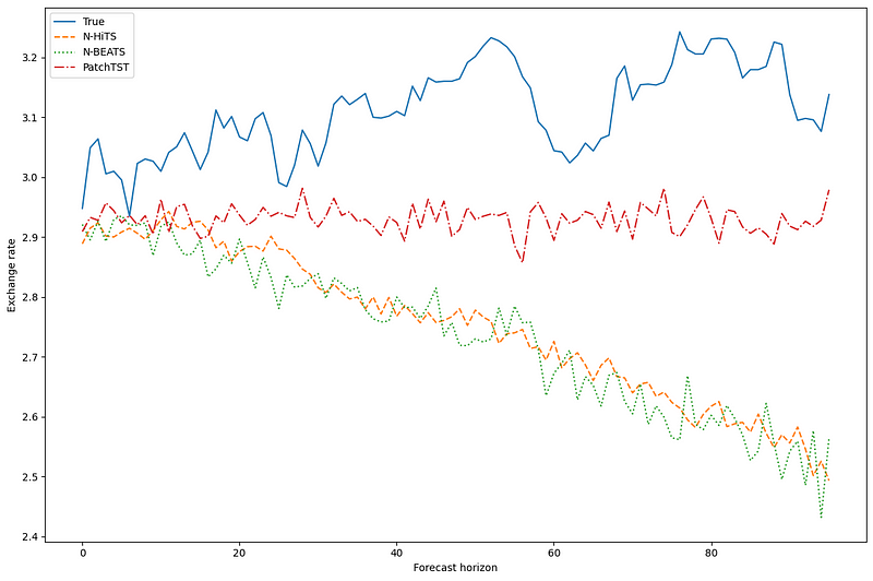
This figure is a bit underwhelming, as N-BEATS and N-HiTS seem to have predictions that are very off from the actual values. However, PatchTST, while also off, seems to be the closest to the actual values.

Of course, we must takes this with a grain of salt, because we are only visualizing the prediction for one series, in one prediction window. 

Evaluation

So, let’s evaluate the performance of each model. To replicate the methodology from the paper, we use both the MAE and MSE as performance metrics.

data = {'N-HiTS': [mae(y_pred_nhits, y_true), mse(y_pred_nhits, y_true)],
       'N-BEATS': [mae(y_pred_nbeats, y_true), mse(y_pred_nbeats, y_true)],
       'PatchTST': [mae(y_pred_patchtst, y_true), mse(y_pred_patchtst, y_true)]}

metrics_df = pd.DataFrame(data=data)
metrics_df.index = ['mae', 'mse']

metrics_df.style.highlight_min(color='lightgreen', axis=1)

In the table above, we see that PatchTST is the champion model as it achieves the lowest MAE and MSE.

Of course, this was not the most thorough experiment, as we only used one dataset and one forecast horizon. Still, it is interesting to see that a Transformer-based model can compete with state-of-the-art MLP models.

Conclusion

PatchTST is a Transformer-based models that uses patching to extract local semantic meaning in time series data. This allows the model to be faster to train and to have a longer input window.

It has achieved state-of-the-art performances when compared to other Transformer-based models. In our little exercise, we saw that it also achieved better performances than N-BEATS and N-HiTS.

While this does not mean that it is better than N-HiTS or N-BEATS, it remains an interesting option when forecasting on a long horizon.

Thanks for reading! I hope that you enjoyed it and that you learned something new!

Cheers 🍻

Support me

Enjoying my work? Show your support with Buy me a coffee, a simple way for you to encourage me, and I get to enjoy a cup of coffee! If you feel like it, just click the button below 👇

References

A Time Series is Worth 64 Words: Long-Term Forecasting with Transformers by Nie Y., Nguyen N. et al.

Neuralforecast by Olivares K., Challu C., Garza F., Canseco M., Dubrawski A.