Lag-Llama: Open-Source Foundation Model for Time Series Forecasting

In October 2023, I published an article on TimeGPT, one of the first foundation model for time series forecasting, capable of zero-shot inference, anomaly detection and conformal prediction capabilities.

However, TimeGPT is a proprietary model that is only accessed via an API token. Still, it sparked more research in foundation models for time series, as this area has been lagging compared to natural language processing (NLP) and computer vision.

Fast-forward to February 2024, and we now have an open-source foundation model for time series forecasting: Lag-Llama.

In the original paper: Lag-Llama: Towards Foundation Models for Probabilistic Time Series Forecasting, the model is presented as a general-purpose foundation model for univariate probabilistic forecasting. It was developed by a large team from different institutions like Morgan Stanley, ServiceNow, Université de Montréal, Mila-Quebec, and McGill University.

In this article, we explore the architecture of Lag-Llama, its capabilities and how it was trained. Then we actually use Lag-Llama in a forecasting project, and compare its performance to other deep learning methods life Temporal Fusion Transformer (TFT) and DeepAR.

Of course, for more details, you can read the original paper.

Learn the latest time series analysis techniques with my free time series cheat sheet in Python! Get the implementation of statistical and deep learning techniques, all in Python and TensorFlow!

Let’s get started!

Explore Lag-Llama

As mentioned earlier, Lag-Llama is built for univariate probabilistic forecasting. 

It uses a general method for tokenizing time series data that does not rely on frequency. That way, the model can generalize well to unseen frequencies.

It leverages the Transformer architecture along with a distribution head to parse the input tokens and map them to future forecasts with confidence intervals.

Since there is a lot to cover, let’s explore each main component in more detail.

Tokenization with lag features

The tokenization strategy of Lag-Llama involves constructing lagged features of the series using a specified set of lags.

Specifically, it will choose all appropriate frequencies for a given dataset from this list:

• quarterly
• monthly
• weekly
• daily
• hourly
• every second

This means that if we feed a dataset with a daily frequency, Lag-Llama will attempt to build features using a daily lag (t-1), a weekly lag (t-7), a monthly lag (t-30), and so on.

This strategy is depicted in the image below.

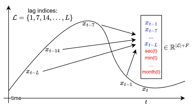
From the figure above, we also notice that other static covariates are built, such as second-of-minute, hour-of-day, and so on, up until quarter-of-year.

While this generalizes well to all kinds of time series, it also comes with the downside that the input token can get very large due to the fixed list of lag indices. 

For example, looking at the monthly frequency of hourly data requires 730 time steps. This means that the input token has a length of at least 730, in addition to all static covariates.

Architecture of Lag-Llama

Lag-Llama is a decoder-only Transformer-based model, and takes inspiration from the architecture of the large language model LLaMA.

A schematic of the architecture is shown below.

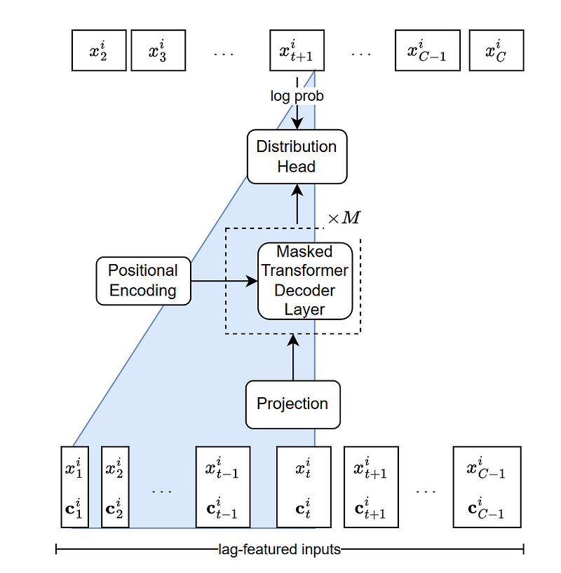
From the figure above, we can see that the input token is a concatenation of lagged time steps and static covariates. 

The input sequence is sent through a linear projection layer that maps the features to a hidden dimension of the attention module inside the decoder.

From there, the input sequence is sent to a distribution head, which is responsible for outputting a probability distribution.

During inference, the input sequence generates the distribution for the next point in time. Then, by autoregressive decoding, the model generates the rest of the forecast sequence until the length of the horizon is reached.

The autoregressive process of generating predictions effectively allows the model to generate uncertainty intervals for its forecasts.

Thus, we can see that the distribution head plays an important role in Lag-Llama, so let’s explore it further.

Understand the distribution head of Lag-Llama

As mentioned above, the distribution head of Lag-Llama is responsible for outputting a probability distribution.

This is how the model is able to generate prediction intervals.

In this iteration of the model, the last layer uses the Student’s t-distribution to construct the uncertainty intervals.

Technically, different distribution heads could be combined, but this experiment was not conducted and is left for future work.

Now that we have a deeper understanding of the inner workings of Lag-Llama, let’s see how the model was trained.s

Training Lag-Llama

Being a foundation model, Lag-Llama was obviously trained on a large corpus of time series data, such that the model can then generalize well on unseen time series and perform zero-shot forecasting.

In this case, Lag-Llama was trained on 27 time series datasets from different domains, such as energy, transportation, economics, and others. 

The training corpus thus contains 7965 univariate time series, totalling around 352 million tokens. 

All datasets are open-source, and include popular benchmarks like Etth, Exchange and Weather.

Note that the datasets were split into a training and test set, allowing the authors to use open-source data to train and evaluate the model. 

 You can consult the full list of datasets used for training here.

Let’s now apply Lag-Llama in small forecasting project.

Forecasting with Lag-Llama

In this small forecasting project, we first use Lag-Llama’s zero-shot forecasting capabilities and compare its performance to data-specific models such as TFT and DeepAR.

It seems that the implementation of Lag-Llama was built on top of GluonTS, so we use this library for this experiment.

Specifically, we use the Australian Electricity Demand dataset, which contains five univariate time series tracking the energy demand at a half-hourly frequency. The dataset is publicly available on the Monash Forecasting Repository.

Note that the current implementation of Lag-Llama is very early. The repository is still being actively developed, and more scripts will be added for more advanced usage, like fine-tuning the model on a dataset.

As always, the full source code for this experiment is available on GitHub.

Environment setup

To use Lag-Llama, we must first clone the repository and install the necessary requirements. 

!git clone https://github.com/time-series-foundation-models/lag-llama/ 

cd lag-llama 

pip install -r requirements.txt --quiet 

Once the packages are installed, we can download the weights of the model from HuggingFace.

!huggingface-cli download time-series-foundation-models/Lag-Llama lag-llama.ckpt --local-dir /content/lag-llama 

Load the dataset

Now, we can load the dataset and prepare it for inference.

We start off with the required library imports.

import pandas as pd 
import matplotlib.pyplot as plt 
import matplotlib.dates as mdates 
import torch

from itertools import islice

from gluonts.evaluation import make_evaluation_predictions, Evaluator 
from gluonts.dataset.repository.datasets import get_dataset 
from lag_llama.gluon.estimator import LagLlamaEstimator 

Then, we can load the dataset directly from GluonTS.

dataset = get_dataset("australian_electricity_demand") 
backtest_dataset = dataset.test prediction_length = dataset.metadata.prediction_length 
context_length = 3 * prediction_length 

The data is now ready to be used for inference.

Predict with Lag-Llama

Then, we can simply initialize the model and use the LagLlamaEstimator object.

ckpt = torch.load("lag-llama.ckpt", map_location=torch.device('cuda:0')) 
estimator_args = ckpt["hyper_parameters"]["model_kwargs"] 

estimator = LagLlamaEstimator( ckpt_path="lag-llama.ckpt", 
  prediction_length=prediction_length, 
  context_length=context_length, 
  input_size=estimator_args["input_size"], 
  n_layer=estimator_args["n_layer"], 
  n_embd_per_head=estimator_args["n_embd_per_head"], 
  n_head=estimator_args["n_head"], 
  scaling=estimator_args["scaling"], 
  time_feat=estimator_args["time_feat"]) 

lightning_module = estimator.create_lightning_module() 
transformation = estimator.create_transformation() 
predictor = estimator.create_predictor(transformation, lightning_module) 

Perfect! We then generate zero-shot predictions using the make_evaluation_predictions function.

forecast_it, ts_it = make_evaluation_predictions(
  dataset=backtest_dataset, 
  predictor=predictor) 

Note that this function returns generators. So, let’s convert them to lists so it’s easier to work with.

forecasts = list(forecast_it) 
tss = list(ts_it) 

Evaluation of Lag-Llama

GluonTS can then conveniently compute different performance metrics using the Evaluator object.

evaluator = Evaluator() 

agg_metrics, ts_metrics = evaluator(iter(tss), iter(forecasts))

Here, we get a RMSE of 481.57. 

Optionally, we can also visualize the predictions. For convenience, we only show the first four series of the dataset.

plt.figure(figsize=(20, 15)) 
date_formater = mdates.DateFormatter('%b, %d') 
plt.rcParams.update({'font.size': 15}) 

for idx, (forecast, ts) in islice(enumerate(zip(forecasts, tss)), 4): 
  ax = plt.subplot(2, 2, idx+1) 
  plt.plot(ts[-4 * dataset.metadata.prediction_length:].to_timestamp(), label="target") 
  forecast.plot( color='g')
 
  plt.xticks(rotation=60) 
  ax.xaxis.set_major_formatter(date_formater) 
  ax.set_title(forecast.item_id) 

plt.gcf().tight_layout() 
plt.legend() 
plt.show() 

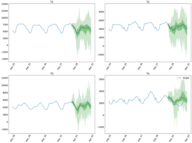
In the figure above, we can see that the model made reasonable predictions on the data, although it does have trouble with the fourth series (bottom right of the figure).

Plus, since Lag-Llama implements probabilistic predictions, we also get uncertainty intervals along with the predictions.

Now that we know how to use Lag-Llama for zero-shot forecasting, let’s compare its performance against data-specific models.

Comparing to TFT and DeepAR

For consistency, we keep using the GluonTS library and train a TFT and DeepAR models on the dataset to see if they can perform better.

To save some time, we constrain training to five epochs only. 

from gluonts.torch import TemporalFusionTransformerEstimator, DeepAREstimator 

tft_estimator = TemporalFusionTransformerEstimator(
  prediction_length=prediction_length, 
  context_length=context_length, 
  freq="30min", 
  trainer_kwargs={"max_epochs": 5}) 

deepar_estimator = DeepAREstimator(
  prediction_length=prediction_length, 
  context_length=context_length, 
  freq="30min", 
  trainer_kwargs={"max_epochs": 5}) 

Once the models are initialized, we can launch the training procedure.

tft_predictor = tft_estimator.train(dataset.train) 
deepar_predictor = deepar_estimator.train(dataset.train) 

Once trained, we generate predictions and calculate the RMSE.

# Make predictions

tft_forecast_it, tft_ts_it = make_evaluation_predictions(
  dataset=backtest_dataset, 
  predictor=tft_predictor) 

deepar_forecast_it, deepar_ts_it = make_evaluation_predictions(
  dataset=backtest_dataset, 
  predictor=deepar_predictor) 

tft_forecasts = list(tft_forecast_it) 
tft_tss = list(tft_ts_it) 

deepar_forecasts = list(deepar_forecast_it) 
deepar_tss = list(deepar_ts_it) 

# Get evaluation metrics
tft_agg_metrics, tft_ts_metrics = evaluator(iter(tft_tss), iter(tft_forecasts)) 
deepar_agg_metrics, deepar_ts_metrics = evaluator(iter(deepar_tss), iter(deepar_forecasts)) 

The table below highlights the best performing model.

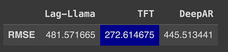
From the table above, we can see that TFT is by far the best performing model, and DeepAR also beats the performance of Lag-Llama.

While the performance of Lag-Llama seems underwhelming, keep in mind that the model was not fine-tuned, and zero-shot forecasting is inherently harder.

On the other hand, the data-specific models were only trained for five epochs, which is interesting to see that both achieve better results than Lag-Llama. While zero-shot forecasting can save time, I would argue that training for five epochs is not demanding in terms of both time and computation power.

Still, we must keep in mind that Lag-Llama is in its early stage, and when fine-tuning capabilities become available, the model is likely going to perform better.

Also, this is far from being an exhaustive benchmark of Lag-Llama, so make sure to test it against other methods for a particular project.

My take on TimeGPT vs Lag-Llama

To me, it seems that we are witnessing in time series what happened a few months ago in NLP.

Proprietary large language models generally perform better than their open-source counterparts, alhtough the open-source models are catching up.

I believe we can draw a similar parallel here. Having tried both TimeGPT and Lag-Llama, the latter seems like a great first step in building an open-source foundation forecasting model, but it falls short in terms of capabilities when compared to TimeGPT.

At the moment, TimeGPT can handle multivariate time series, irregular timestamps, and it implements conformal predictions, which is a more robust way of quantifying uncertainty compared to using a fixed distribution like in Lag-Llama.

Nevertheless, I believe we are going to see more open-source foundation forecasting models appear in the near future. Their performance is likely going to improve, and that represents a big paradigm shift for the field. 

In brief, we are going through exciting times in the field of forecasting.

Conclusion

Lag-Llama is an open-source foundation model for univariate probabilistic forecasting. 

It uses a decoder-only Transformer architecture with a distribution head to generate probabilistic predictions, meaning that we get uncertainty intervals immediately.

The model implements a general tokenization strategy that involves creating lagged features and constructing static covariates, such as time-of-day, day-of-week, etc.

It is built on top of GluonTS, so for now, we have to use that library to actually generate predictions from Lag-Llama.

As always, I think that each problem requires its unique solution. Make sure to test Lag-Llama against other methods.

Thanks for reading! I hope that you enjoyed it and that you learned something new!

Looking to master time series forecasting? Then check out my course Applied Time Series Forecasting in Python. This is the only course that uses Python to implement statistical, deep learning and state-of-the-art models in 16 guided hands-on projects.

Cheers 🍻

Support me

Enjoying my work? Show your support with Buy me a coffee, a simple way for you to encourage me, and I get to enjoy a cup of coffee! If you feel like it, just click the button below 👇

References

Lag-Llama: Towards Foundation Models for Probabilistic Time Series Forecasting by K. Rasul, A. Ashok, A. Williams, H. Ghonia, R. Bhagwatkar, A. Khorasani, M. Bayazi, G. Adamopoulos, R. Riachi, N. Hassen, M. Bilos, S. Garg, A. Schneider, N. Chapados, A. Drouin, V. Zantedeschi, Y. Nevmyvaka, I. Rish

Original repository of Lag-Llama — GitHub