iTransformer: The Latest Breakthrough in Time Series Forecasting

The field of forecasting has seen a lot of activity in the realm of foundation models, with models like Lag-LLaMA, Time-LLM, Chronos and Moirai being proposed since the beginning of 2024. 

However, their performance has been a bit underwhelming (for reproducible benchmarks, see here), and I believe that data-specific models are still the optimal solution at the moment.

To that end, the Transformer architecture has been applied in many forms for time series forecasting, with PatchTST achieving state-of-the-art performance for long-horizon forecasting.

Challenging PatchTST comes the iTransformer model, proposed in March 2024 in the paper iTransformer: Inverted Transformers Are Effective for Time Series Forecasting.

In this article, we discover the strikingly simple concept behind iTransformer and explore its architecture. Then, we apply the model in a small experiment and compare its performance to TSMixer, N-HiTS and PatchTST.

For more details, make sure to read the original paper.

Let’s get started!

Explore iTransformer

The idea behind iTransformer comes from the realization that the vanilla Transformer model uses temporal tokens.

This means that the model looks at all features at a single time step. Thus, it is challenging for the model to learn temporal dependencies when looking at one time step at a time.

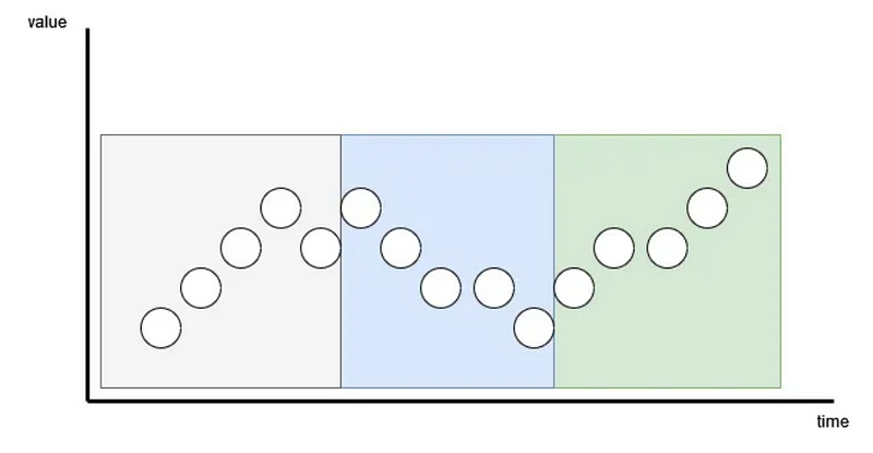
A solution to that problem is patching, which was proposed with the PatchTST model. With patching, we simply group time points together before tokenizing and embedding them, as shown below.

In iTransformer, we push patching to the extreme by simply applying the model on the inverted dimensions. 

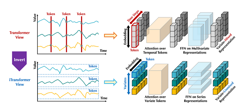
In the figure above, we can see how the iTransformer differs from the vanilla Transformer. Instead of looking at all features at one time step, it looks at one feature across many time steps. This is done simply by inverting the shape of the input.

This way, the attention layer can learn multivariate correlations and the feed-forward network encodes the representation of the whole input sequence.

Now that we grasp the general idea behind iTransformer, let’s take a look at its architecture in more detail.

Architecture of iTransformer

The iTransformer employs the vanilla encoder-decoder architecture with the embedding, projection and Transformer blocks, as originally proposed in the seminal paper Attention Is All You Need in 2017.

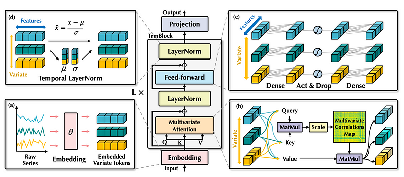
From the figure above, we can see that the building blocks are the same, but their function is entirely different. Let’s take a closer look.

Embedding layer

First, the input series are independently embedded as tokens. Again, this is like an extreme case of patching, where instead of tokenizing subsequences of the input, the model tokenizes the entire input sequence.

Multivariate attention

Then, the embeddings are sent to the attention layer, where it will learn a multivariate correlation map. 

This is possible because the inverted model sees each feature as an independent process. As a result, the attention mechanism learns correlations between pairs of features, making iTransformer especially suitable for multivariate forecasting tasks.

Layer normalization

The output of the attention layer is sent to the normalization layer. 

In the traditional Transformer architecture, normalization is done for all features at a fixed timestamp. This can introduce interaction noise, meaning that the model is learning useless relationships. Plus, it can result in an overly smooth signal.

By contrast, since iTransformer inverts the dimensions, normalization is done across timestamps. This helps the model tackle non-stationary series, and it reduces the noise in the series.

Feed-forward network

Finally, the feed-forward network (FFN) learn a deep representation of the incoming tokens. 

Again, since the shapes are inverted, the multilayer perceptron (MLP) can learn different temporal properties, like periodicity and amplitude. This mimics the capabilities of MLP-based models, like N-BEATS, N-HiTS and TSMixer.

Projection

From here, it is simply a matter of stacking many blocks composed of:

• attention layer
• layer normalization
• feed-forward network
• layer normalization

Each block learns a different representation of the input series. Then, the output of the stack of blocks is sent through a linear projection step to obtain the final forecasts.

In summary, the iTransformer is not a new architecture; it does not reinvent the Transformer. It simply applies it on the inverted dimensions of the input, which allows the model to learn multivariate correlations and capture temporal properties.

Now that we have a deep understanding of the iTransformer model, let’s apply it in a small forecasting experiment.

Forecasting with iTransformer

For this small experiment, we apply the iTransformer model on Electricity Transformer dataset released under the Creative Commons License.

This is a popular benchmark dataset that tracks the oil temperature of an electricity transformer from two regions in a province of China. For both regions, we have a dataset sampled at each hour and every 15 minutes, for a total of four datasets.

While the iTransformer is fundamentally a multivariate model, we test its univariate forecasting capabilities on a horizon of 96 time steps.

The code for this experiment is available on GitHub.

Let’s get started!

Initial setup

For this experiment, we use the library neuralforecast, as I believe it provides the fastest and most intuitive ready-to-use implementations of deep learning methods.

import pandas as pd
import numpy as np
import matplotlib.pyplot as plt

from datasetsforecast.long_horizon import LongHorizon

from neuralforecast.core import NeuralForecast
from neuralforecast.models import NHITS, PatchTST, iTransformer, TSMixer

Note that at the time of writing this article, iTransformer is not available in a public release of neuralforecast just yet. To access the model immediately you can run:

pip install git+https://github.com/Nixtla/neuralforecast.git

Now, let’s write a function to load the ETT datasets, along with their validation size, test size, and frequency.

def load_data(name):
    if name == "ettm1":
        Y_df, *_ = LongHorizon.load(directory='./', group='ETTm1')
        Y_df = Y_df[Y_df['unique_id'] == 'OT']
        Y_df['ds'] = pd.to_datetime(Y_df['ds'])
        val_size = 11520
        test_size = 11520
        freq = '15T'
    elif name == "ettm2":
        Y_df, *_ = LongHorizon.load(directory='./', group='ETTm2')
        Y_df = Y_df[Y_df['unique_id'] == 'OT']
        Y_df['ds'] = pd.to_datetime(Y_df['ds'])
        val_size = 11520
        test_size = 11520
        freq = '15T'
    elif name == 'etth1':
        Y_df, *_ = LongHorizon.load(directory='./', group='ETTh1')
        Y_df['ds'] = pd.to_datetime(Y_df['ds'])
        val_size = 2880
        test_size = 2880
        freq = 'H'
    elif name == "etth2":
        Y_df, *_ = LongHorizon.load(directory='./', group='ETTh2')
        Y_df['ds'] = pd.to_datetime(Y_df['ds'])
        val_size = 2880
        test_size = 2880
        freq = 'H'

    return Y_df, val_size, test_size, freq

The function above conveniently loads the data in the format expected by neuralforecast, where we have a unique_id column to label unique time series, a ds column for the timestamp, and a y column with the value of our series.

Also note that the validation and test sizes are consistent with what the scientific community uses when publishing their papers.

We are now ready to train the models.

Training and forecasting

To train the iTransformer model, we simply need to specify the:

• forecast horizon
• input size
• number of series

Remember that iTransformer is fundamentally a multivariate model, which is why we need to specify the number of series when fitting the model.

Since we are in a univariate scenario, n_series=1.

iTransformer(h=horizon, 
             input_size=3*horizon, 
             n_series=1, 
             max_steps=1000, 
             early_stop_patience_steps=3)

In the code block above, we also specify the maximum number of training steps, and we set early stopping to three iterations to avoid overfitting.

We then do the same for the other models, and place them in a list.

horizon = 96

models = [
    iTransformer(h=horizon, input_size=3*horizon, n_series=1, max_steps=1000, early_stop_patience_steps=3),
    TSMixer(h=horizon, input_size=3*horizon, n_series=1, max_steps=1000, early_stop_patience_steps=3),
    NHITS(h=horizon, input_size=3*horizon, max_steps=1000, early_stop_patience_steps=3),
    PatchTST(h=horizon, input_size=3*horizon, max_steps=1000, early_stop_patience_steps=3)
]

Great! Now, we simply initialize the NeuralForecast object which gives access to methods for training, cross-validation, and making predictions.

nf = NeuralForecast(models=models, freq=freq)
nf_preds = nf.cross_validation(df=Y_df, val_size=val_size, test_size=test_size, n_windows=None)

Finally, we evaluate the performance of each model using the utilsforecast library.

from utilsforecast.losses import mae, mse
from utilsforecast.evaluation import evaluate

ettm1_evaluation = evaluate(df=nf_preds, metrics=[mae, mse], models=['iTransformer', 'TSMixer', 'NHITS', 'PatchTST'])
ettm1_evaluation.to_csv('ettm1_results.csv', index=False, header=True)

These steps are then repeated for all datasets. The complete function to run this experiment is shown below.

from utilsforecast.losses import mae, mse
from utilsforecast.evaluation import evaluate

datasets = ['ettm1', 'ettm2', 'etth1', 'etth2']

for dataset in datasets:

    Y_df, val_size, test_size, freq = load_data(dataset)
    
    horizon = 96
    
    models = [
        iTransformer(h=horizon, input_size=3*horizon, n_series=1, max_steps=1000, early_stop_patience_steps=3),
        TSMixer(h=horizon, input_size=3*horizon, n_series=1, max_steps=1000, early_stop_patience_steps=3),
        NHITS(h=horizon, input_size=3*horizon, max_steps=1000, early_stop_patience_steps=3),
        PatchTST(h=horizon, input_size=3*horizon, max_steps=1000, early_stop_patience_steps=3)
    ]
    
    nf = NeuralForecast(models=models, freq=freq)
    nf_preds = nf.cross_validation(df=Y_df, val_size=val_size, test_size=test_size, n_windows=None)
    nf_preds = nf_preds.reset_index()
    
    evaluation = evaluate(df=nf_preds, metrics=[mae, mse], models=['iTransformer', 'TSMixer', 'NHITS', 'PatchTST'])
    evaluation.to_csv(f'{dataset}_results.csv', index=False, header=True)

Once this is done running, we have predictions from all of our models on all datasets. We can then move on to evaluation.

Performance evaluation

Since we saved all performance metrics in CSV files, we can read them using pandas and plot the performance of each model for each dataset.

files = ['etth1_results.csv', 'etth2_results.csv', 'ettm1_results.csv', 'ettm2_results.csv']
datasets = ['etth1', 'etth2', 'ettm1', 'ettm2']

dataframes = []

for file, dataset in zip(files, datasets):
    df = pd.read_csv(file)
    df['dataset'] = dataset

    dataframes.append(df)

full_df = pd.concat(dataframes, ignore_index=True)
full_df = full_df.drop(['unique_id'], axis=1)

Then, to plot the metrics:

import matplotlib.pyplot as plt
import numpy as np

dataset_names = full_df['dataset'].unique()
model_names = ['iTransformer', 'TSMixer', 'NHITS', 'PatchTST']

fig, axs = plt.subplots(2, 2, figsize=(15, 15)) 
bar_width = 0.35  

axs = axs.flatten()

for i, dataset_name in enumerate(dataset_names):
    df_subset = full_df[(full_df['dataset'] == dataset_name) & (full_df['metric'] == 'mae')]
    mae_vals = df_subset[model_names].values.flatten()
    df_subset = full_df[(full_df['dataset'] == dataset_name) & (full_df['metric'] == 'mse')]
    mse_vals = df_subset[model_names].values.flatten()
    
    indices = np.arange(len(model_names))
    
    bars_mae = axs[i].bar(indices - bar_width / 2, mae_vals, bar_width, color='skyblue', label='MAE')
    bars_mse = axs[i].bar(indices + bar_width / 2, mse_vals, bar_width, color='orange', label='MSE')
    
    for bars in [bars_mae, bars_mse]:
        for bar in bars:
            height = bar.get_height()
            axs[i].annotate(f'{height:.2f}', 
                            xy=(bar.get_x() + bar.get_width() / 2, height),
                            xytext=(0, 3),
                            textcoords="offset points",
                            ha='center', va='bottom')
    
    axs[i].set_xticks(indices)
    axs[i].set_xticklabels(model_names, rotation=45)
    axs[i].set_title(dataset_name)
    axs[i].legend(loc='best')

plt.tight_layout()

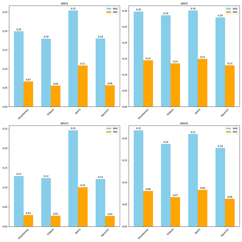
From the figure above, we can see that the iTransformer performs fairly well on all datasets, but TSMixer is overall slightly better than iTransformer, and PatchTST is the overall champion model in this experiment.

Of course, keep in mind that we did not leverage the multivariate capabilities of iTransformer, and we only tested on a single forecast horizon. Therefore, it is not a complete assessment of the iTransformer’s performance.

Nevertheless, it is interesting to see the model perform very closely to PatchTST, which further supports the idea that grouping time steps together before tokenizing unlocks new heights in performance when using Transformers for time series forecasting.

Conclusion

The iTransformer takes the vanilla Transformer architecture and simply applies it to the inverted shape of the input series.

That way, the entire series is tokenized, which mimics an extreme case of patching, as proposed in PatchTST.

This allows the model to learn multivariate correlations using its attention mechanism, while the feed-forward network learn temporal properties of the series.

The iTransformer was shown to achieve state-of-the-art performance for long-horizon forecasting on many benchmark datasets, although in our limited experiment, PatchTST performed best overall. 

I firmly believe that every problem requires its unique solution, and now you can add the iTransformer to your toolbox and apply it in your projects.

Thanks for reading! I hope that you enjoyed it and that you learned something new!

Looking to master time series forecasting? The check out Applied Time Series Forecasting in Python. This is the only course that uses Python to implement statistical, deep learning and state-of-the-art models in 15 guided hands-on projects.

Cheers 🍻

Support me

Enjoying my work? Show your support with Buy me a coffee, a simple way for you to encourage me, and I get to enjoy a cup of coffee! If you feel like it, just click the button below 👇

References

iTransformer: Inverted Transformers Are Effective for Time Series Forecasting by Yong Liu, Tengge Hu, Haoran Zhang, Haixu Wu, Shiyu Wang, Lintao Ma, Mingsheng Long