Introduction to Causal Inference with Machine Learning in Python

Causal inference has many tangible applications in a wide variety of scenarios, but in my experience, it is a subject that is rarely talked about among data scientists.

In this article, we define causal inference and motivate its use. Then, we apply some basic algorithms in Python to measure the effect of a certain phenomenon.

Define causal inference

Causal inference is a field of study interested in measuring the effect of a certain treatment.

Another way to think about causal inference, is that it answers what-if questions. The goal is always to measure some kind of impact given a certain action.

Examples of questions answered with causal inference are:

• What is the impact of running an ad campaign on product sales?
• What is the effect of a price increase on sales?
• Does this drug make patients heal faster?

We can see that these questions are relevant for decision-makers, but they cannot be addressed with traditional machine learning methods.

Causal inference vs traditional machine learning

With traditional machine learning techniques, we generate predictions or forecasts given a set of features.

For example, we can forecast how many sales we would do next month. 

In other words, machine learning models uncover correlations between features and a target to better predict that target. In that sense, any correlation between some feature and the target is useful if it allows the model to make better predictions.

When it comes to causal inference, we wish to measure the impact of a treatment.

For example, we can determine how increasing a product’s price will impact sales.

Thus, with causal inference, we seek to uncover causal pathways.

Correlation is not causation

We often hear that correlation is not causation, and that is a critical point when it comes to causal inference. 

We must be careful to not fall in the trap of spurious correlation. This is a mathematical relationship in which two or more variables are associated, but are not causally related.

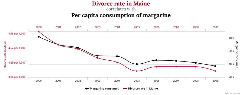
In the figure above, we can see an example of a spurious relationship. Clearly, the divorce rate in Maine and the per capita consumption of margarine are correlated, but there is no causal pathway.

In theory, a machine learning model could use one variable to predict the other and it would likely help the model make better predictions (in practice, we still want to avoid spurious relationships in ML models).

However, in the realm of causal inference, we have to identify the causal pathway before applying our model, to make sure that we are measuring the true impact from the cause.

Uncover causal pathways

Now, we should be convinced that for causal inference to make sense, we need a human to draw the causal pathway, so that we can understand the effect of a treatment on a certain outcome.

To help us draw the causal chain, let’s consider the following scenario:

You are an ice cream vendor and you want to know the impact of offering a discount on ice cream sales.

The causal pathway can be visualized like so:

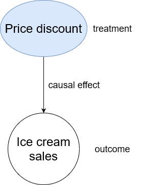
From the figure above, we can see the simple causal pathway for our scenario. 

Because the causal chain is so simple, this is a good time to introduce some nomenclature used in causal inference.

In the figure, offering a discount is called the treatment (denoted as the variable T in equations). Here, it could mean that instead of selling an ice cream for $2, we offer it at $1.50.

This potentially has some effect on the ice cream sales. This is designated as the outcome (denoted as Y in equations). 

Now, offering a discount is not the only element impacting ice cream sales. 

For example, consider the fact that we may have returning customers. Returning customers probably like ice cream and they would buy it, no matter the discount. Similarly, returning customers are more likely to see the discount. 

As we can see, a returning customer is related to both the treatment and the outcome. This is what we call a confounder.

Understand confounders

A confounder is a variable that influences both the treatment and the outcome. 

In the previous section, we identified that whether a customer is a repeat customer or not is a confounding variable.

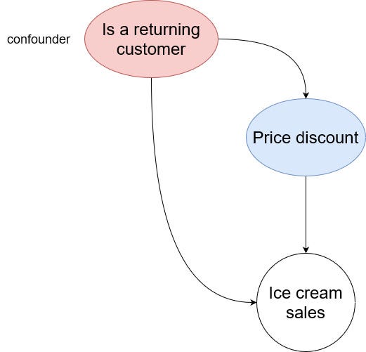
From the figure above, we can see that the confounder influences both the treatment and the outcome. Therefore, it can introduce a bias when measuring the treatment effect.

It is thus important to identify confounders and to learn how to appropriately deal with them to measure the treatment effect as precisely as possible. 

Such techniques are explored in the next section.

Measure the treatment effect

Until now, we know that causal inference helps us measure the treatment effect on a certain outcome, but we have to watch out for confounders, as they can introduce a bias in our measurement.

To measure the treatment effect, there are three broad methods:

1. Randomized experiments
2. Measure confounders
3. Instrument variables

Let’s explore each one in more detail.

Randomized experiments

Randomized experiments are referred to as the gold standard when it comes to measuring the treatment effect.

In essence, it is a fairly simple method: simply assign the treatment at random. 

That way, any effect from the confounders on the treatment is removed as shown below.

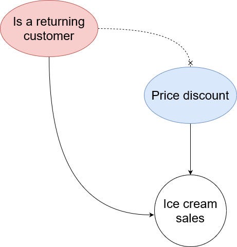
Since the confounder does not influence getting the treatment anymore, any change we see between the treated (customers who got a discount) and untreated (customers who don’t get a discount) is the causal treatment effect.

The major advantage of this method is that we do not need to worry about confounding variables anymore, and it completely isolates the causal effect.

However, in reality, it is not always possible to run this kind of experiment. For example, a company cannot possibly offer discounts at random, as it could impact its reputation. 

Measure confounders

Another way of measuring the causal effect is to actually measure (or control) the confounding variables.

That way, it is possible to measure the effect of the confounder on the treatment, and then isolate the effect of the treatment on the outcome.

This has the advantage of being applicable on observational data without the need for an experiment. 

However, it requires identifying and measuring all confounders, which again is not always possible. 

Instrument variables

Instrument variables are used when we cannot create a randomized experiment and when we have confounders that cannot be measured.

By definition, an instrument variable has an effect on the treatment, but not on the outcome.

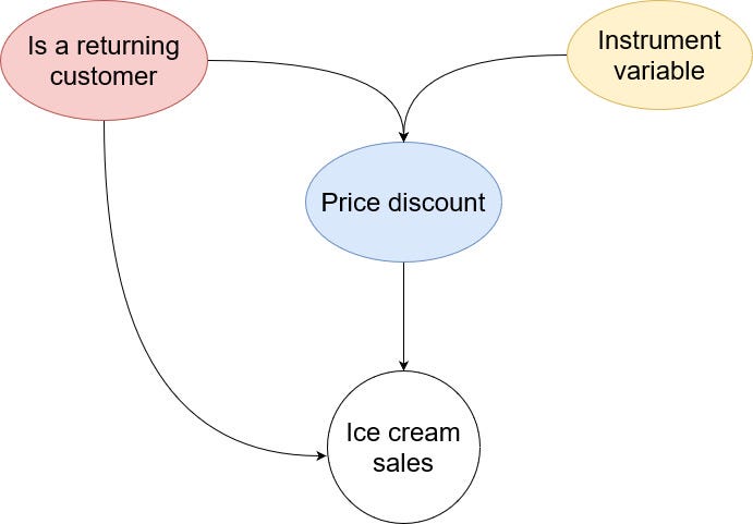
Since we assume that the instrument variable is not linked to the outcome, any correlation between the instrument and the outcome has to come through the treatment.

In our ice cream sales scenario, maybe that we have different managers running the ice cream shop and not all of them offer a discount. In this case, the manager can be used as an instrument variable.

The main advantages of this method is that it works on observational data and we do not need to account for all confounders.

On the other hand, finding good instrument variables is very hard. In fact, we might be at risk of introducing more bias in our measurement if the instrument is only weakly linked to the treatment.

Now that we have explored all methods of measuring the treatment effect, let’s apply our knowledge in Python.

Applied causal inference

Let’s apply what we have learned to measure the treatment effect using Python.

Here, we use a simulated dataset, so that we know what the actual treatment value is, making it easier to evaluate the performance of our estimation methods.

As always, the entire source code for this experiment is on GitHub.

Now, let’s import the required libraries for this section.

import numpy as np
import pandas as pd
import seaborn as sns
import matplotlib.pyplot as plt

import dowhy
from dowhy import CausalModel
import dowhy.datasets

import warnings
warnings.filterwarnings('ignore')

Then, we generate the synthetic data. Here, we have a treatment effect value of 8. Then, we add two confounders, two instrument variables, and one feature. Finally, we generate 5000 samples and store them in a DataFrame.

Note that the treatment is binary, meaning that you either get the treatment or not.

BETA = 8

data = dowhy.datasets.linear_dataset(BETA,
                                    num_common_causes=2, # confounders
                                    num_samples=5000,
                                    num_instruments=2, # instrument variables
                                    num_effect_modifiers=1, # features
                                    treatment_is_binary=True,
                                    stddev_treatment_noise=5,
                                    num_treatments=1)

df = data['df']

Optionally, we can visualize the distribution of the target according to the treatment, which gives us an idea of any causal impact.

plt.figure(figsize=(6,5))

sns.boxplot(y='y', x='v0', data=df)

plt.tight_layout()

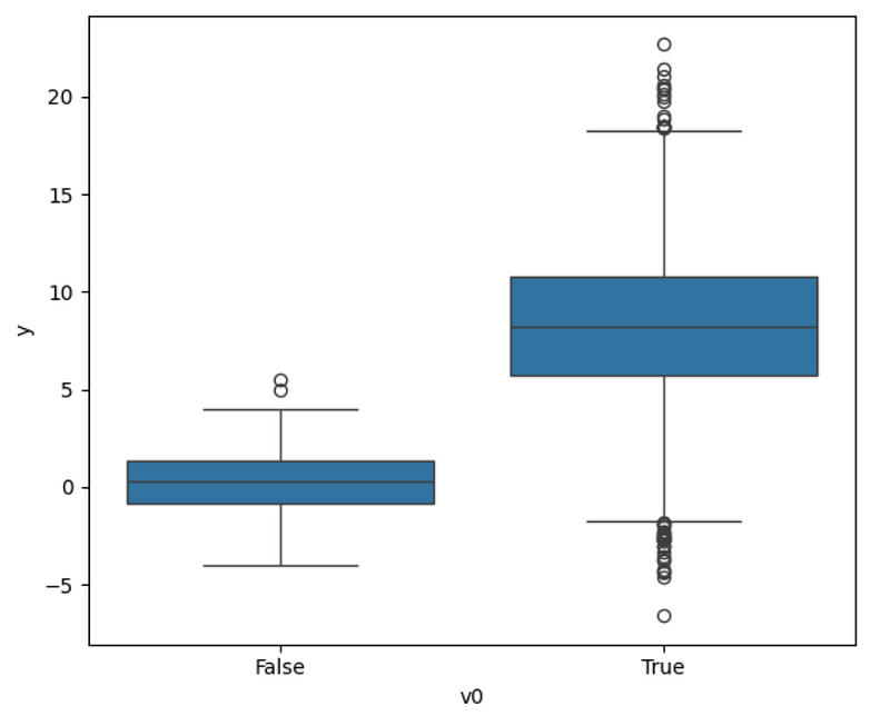
From the figure above, we can indeed see that the treated group has a higher average than the untreated group. This is a strong hint of causality, but it is obviously not the most robust method.

Measure the treatment effect with Python

Now, to measure the treatment effect, we use the package dowhy which is part of the PyWhy ecosystem.

Here, we must first identify causal paths and then measure the effect.

To do so, we must create an instance of CausalModel which conveniently comes with plotting capabilities.

model = CausalModel(data=data['df'],
                   treatment=data['treatment_name'],
                   outcome=data['outcome_name'],
                   graph=data['gml_graph'])

model.view_model()

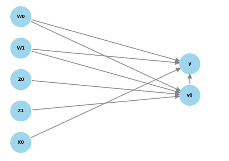
In the figure above, we can see the causal graph of our synthetic dataset.

As expected, we have two confounders (W0 and W1) which have an effect on the treatment (v0) and the outcome (y). We also have two instrument variables (Z0 and Z1) related only to the treatment. Finally, we have one feature (X0) affecting the outcome.

We did not address features in the previous sections, but they are simply variables that impact the outcome directly. In our example of ice cream sales, the temperature could be a feature, since cold temperatures likely mean less ice cream sales, no matter the discount.

With this step complete, we can now identify the different ways of measuring the treatment effect.

identified_estimand= model.identify_effect(proceed_when_unidentifiable=True)

print(identified_estimand)

The output from the code block above is:

### Estimand : 1
Estimand name: backdoor
Estimand expression:
  d              
─────(E[y|W0,W1])
d[v₀]            
Estimand assumption 1, Unconfoundedness: If U→{v0} and U→y then P(y|v0,W0,W1,U) = P(y|v0,W0,W1)

### Estimand : 2
Estimand name: iv
Estimand expression:
 ⎡                              -1⎤
 ⎢    d        ⎛    d          ⎞  ⎥
E⎢─────────(y)⋅⎜─────────([v₀])⎟  ⎥
 ⎣d[Z₀  Z₁]    ⎝d[Z₀  Z₁]      ⎠  ⎦
Estimand assumption 1, As-if-random: If U→→y then ¬(U →→{Z0,Z1})
Estimand assumption 2, Exclusion: If we remove {Z0,Z1}→{v0}, then ¬({Z0,Z1}→y)

### Estimand : 3
Estimand name: frontdoor
No such variable(s) found!

From the output above, we see that we can choose between two methods:

1. Backdoor
2. Instrument variable

Covering the backdoor method is beyond the scope of this article which is meant to be an introduction to the field. Therefore, let’s stick to using the instrument variables.

causal_estimate = model.estimate_effect(
    identified_estimand,
    method_name="iv.instrumental_variable")

print(causal_estimate.value)

This returns a treatment effect of 8.22. Remember that the theoretical value was 8, so this method got very close to measuring the real effect of the treatment.

Causal inference with machine learning

It is also possible to use machine learning methods to estimate the treatment effect.

Here, we implement the Double Machine Learning method or DML. The general idea is to use machine learning models to learn the relationship between the features and the outcome, and between the treatment and the confounders. 

Then, we can remove those relationships to just isolate the effect of the treatment on the outcome.

While any model can be applied in this method, here we use a GradientBoostingRegressor and a final Lasso model to estimate the causal effect.

from sklearn.preprocessing import PolynomialFeatures
from sklearn.linear_model import LassoCV
from sklearn.ensemble import GradientBoostingRegressor

dml_estimate = model.estimate_effect(
    identified_estimand, 
    method_name="iv.econml.dml.DML",
    control_value = 0,
    treatment_value = 1,
    confidence_intervals=False,
    method_params={"init_params":{'model_y':GradientBoostingRegressor(),
                                  'model_t': GradientBoostingRegressor(),
                                  "model_final":LassoCV(fit_intercept=False),
                                  'featurizer':PolynomialFeatures(degree=1, include_bias=False)},
                   "fit_params":{}})
print(dml_estimate.value)

This returns a value of 7.41. Here, we are further from the theoretical value of 8 than what we obtained from the previous method.

Evaluate the model

Remember that in causal inference, we are not making predictions. While we know the correct theoretical value for our synthetic data, in the real world, there is no target, so we cannot report an error metric, like the MAE or the MSE.

Instead, we evaluate the robustness of the model in identifying a causal effect under assumptions violations.

One way to test that is to add a random common cause. In this procedure, we add an independent random variable as a cause of the outcome. Of course, since the variable is random and independent, it should not impact the our measure of the treatment effect.

res_random=model.refute_estimate(identified_estimand, causal_estimate, method_name="random_common_cause")

print(res_random)

This outputs:

Refute: Add a random common cause
Estimated effect:8.218755524405902
New effect:8.218755524405902
p value:1.0

From the output above, we can see that adding a random common cause does not change the measured effect. This is further supported by a p-value of 1. 

We thus conclude that our model is robust and we can trust its causal effect estimate. 

Conclusion

We covered a lot in this article.

We introduced the field of causal inference and realized that unlike in traditional machine learning, we are not doing predictions, but instead measuring the impact of a treatment on an outcome.

We discovered that in real life, many things impact the outcome:

• we have confounders that are related to the treatment and the outcome
• we have features that are related to the outcome directly
• we can add instrument variables that correlate only with the treatment

In brief, methods exist to isolate the treatment effect and remove the bias of confounders and features, but domain knowledge and human inputs remain important to design the right causal graph and then use the right methods.

Finally, we implemented some of those methods using the dowhy package in Python.

There is still so much more to cover on this subject, and I hope that I got you curious to learn more.

Cheers 🍻

Support me

Enjoying my work? Show your support with Buy me a coffee, a simple way for you to encourage me, and I get to enjoy a cup of coffee! If you feel like it, just click the button below 👇

References

DoWhy package — https://www.pywhy.org/dowhy/v0.11.1/

EconML package — https://econml.azurewebsites.net/