Extend N-BEATS for Accurate Time Series Forecasting

The N-BEATS model uses a pure deep learning architecture for time series forecasting. At the time of its release in 2020 [1], this represented an innovative approach, as until then, the best forecasting models usually combined machine learning and statistical models.

In this article, we explore a modification on which Tyler Blume and myself collaborated on. This modification allows users to choose the basis function when modeling with N-BEATS. 

This makes the model more flexible and adaptable to different trends in time series.

While this modification is not an official addition to the model from the original authors, we will see it is a simple feature that can result in more accurate forecasts.

This article assumes some knowledge of N-BEATS, so make sure to explore the inner workings of N-BEATS either with my previous blog article or by reading the original paper.

Let’s get started!

Learn the latest time series forecasting techniques with my 👉 free time series cheat sheet 👈 in Python! Get the implementation of statistical and deep learning techniques, all in Python and TensorFlow!

Quickly revisiting N-BEATS

N-BEATS stands for Neural Basis Expansion Analyis for Interpretable Time Series.

As the name suggests, N-BEATS relies on basis expansion. This is a mathematical operation for augmenting data to model non-linear relationships. 

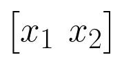
A common approach is using a polynomial basis expansion. For example, suppose that we have only two features, as shown below.

Then, with a basis expansion using a second-degree polynomial, we add the square of each feature to our set, as shown below.

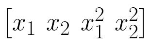
With this new set of feature, we can then fit a second-degree polynomial to our data. 

This is essentially what happens when we fit a line through data in Excel. 

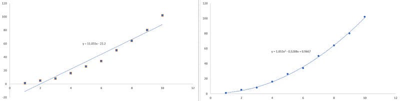
Thus, we can see how using basis expansion helps model different trends in data. While we have shown examples using the polynomial basis, we can use other basis functions like: logarithmic, piecewise linear, and more.

Now, let’s revisit the architecture of N-BEATS before exploring our proposed modification in more detail.

Architecture of N-BEATS

The architecture of N-BEATS is shown in the figure below.

From the figure above, we see that N-BEATS is made of a series of stacks, which are made of blocks.

A block is the basic unit of N-BEATS. We can see it is made of fully-connected layers. We have one fully-connected layer responsible for a forecast, and another for the backcast. 

Here, the forecast represents the prediction of the block, while the backcast represents the learned information by the block. In other words, it is a reconstruction of the input from what the block has learned.

Moving up to the stack, we see that each stack is composed of many
blocks. Again, each stack has two outputs: a prediction and a stack residual. 

The prediction of each stack is summed up and represents a partial forecast at the stack level. Then, the residuals are calculated using the backcast of the block and a residual connection. 

In the figure above, we see a residual connection that completely skips Block 1. This contains the original information coming from the input. Then, the backcast of Block 1 is subtracted from the input. Therefore, Block 2 gets, as an input, the information from the series that was not captured by Block 1. This operation is repeated within a stack, where each block
learns information not captured by previous blocks.

Finally, N-BEATS is made of many stacks, where each output a partial forecast. Their sum represents the final forecast made by N-BEATS.

Now that we have a better understanding of N-BEATS and its inner workings, let’s discover the different types of stacks that can be used in the model. This is a crucial step to understand our proposed modification.

Explore the types of stacks

When using N-BEATS with neuralforecast, we can specify the type of stack. This comes from the model’s capability to have a generic or interpretable architecture as shown below.

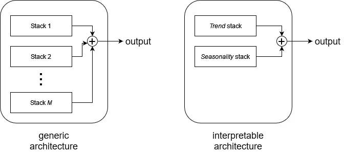
On the left, the generic architecture uses identity stacks. They use the identity basis function which permits the model to learn an arbitrary function that maps the input to the output. As such, it is hard for a human to interpret what is learned by the model.

On the right, the interpretable architecture uses the trend stack and seasonality stack. There, a predefined basis function is used for each stack:

• the trend stack uses a polynomial basis function
• the seasonality stack uses a Fourier basis function

By forcing the model to use a particular basis function, we remove some of its flexibility, but greatly increase the interpretability of the model.

In the available implementation from neuralforecast, we can decide to mix all types of stacks. In other words, we can combine an identity stack with a trend stack and a seasonality stack.

Now, our proposed modification comes within the trend stack where we allow the user to choose from different basis functions to model the trend component.

Choosing different basis functions in the trend stack

While the original method forced a polynomial function in the trend stack, the modification suggested by Tyler Blume and myself gives more flexibility by giving the choice of multiple functions to model the trend.

Specifically, we made available the following functions:

•  polynomial basis
• Legendre polynomial basis
• changepoint basis
• piecewise linear basis
• linear hat basis
• spline basis
• Chebyshev polynomial basis

While simple, this modification allows us to better tailor the trend stack to our data. 

For example, we can use the changepoint basis when notice that the trend abruptly changes in time. Or we can use the piecewise linear basis when the trend changes regime at certain points in time. Other polynomial basis could also result in better performance if they better represent the input data.

Thus, with this simple addition, we can now also tune the basis function used in N-BEATS to model the trend of our data, giving us the opportunity to make more accurate forecasts.

This modification is only available in neuralforecast.

With all of this in mind, let’s see this in action in a small experiment.

Forecasting with N-BEATS while varying the basis function

In this experiment, we use the M3 (by Makridakis and Hibon, 2000) and M4 datasets (by Makridakis et al., 2020), which are available through the Creative Commons Attribution 4.0 license, to test different configurations of N-BEATS. This represents 102 000 unique time series covering yearly, quarterly, monthly, weekly, daily and hourly frequencies.

Here, we compare the performance of using only the identity stack, which learns an arbitrary function, against using the trend and seasonality stack while specifying different basis functions for the trend stack.

That way, we can measure if setting different basis functions can result in more accurate forecasts.

Specifically, we will test the:

• polynomial basis (with different degrees)
• piecewise linear basis (with different breaking points)
• changepoint basis (with different breaking points)

The full code to reproduce the results is available on GitHub. Many thanks to Tyler Blume for setting up the code for the experiments.

Initial setup

As mentioned, this change is only available in neuralforecast, so make sure to install it. We also need utilsforecast to evaluate the performance, and datasetsforecast to load the M3 and M4 datasets.

Then, we can import the required packages.

import pandas as pd

from datasetsforecast.m3 import M3
from datasetsforecast.m4 import M4

from utilsforecast.losses import mae, smape
from utilsforecast.evaluation import evaluate

from neuralforecast import NeuralForecast
from neuralforecast.models import NBEATS

After, we define a function to load the a particular dataset along with its corresponding frequency, forecast horizon, and test sequence.

def get_dataset(name):
    if name == 'M3-yearly':
        Y_df, *_ = M3.load("./data", "Yearly")
        horizon = 6
        freq = 'Y'
    elif name == 'M3-quarterly':
        Y_df, *_ = M3.load("./data", "Quarterly")
        horizon = 8
        freq = 'Q'
    elif name == 'M3-monthly':
        Y_df, *_ = M3.load("./data", "Monthly")
        horizon = 18
        freq = 'M'
    elif name == 'M4-yearly':
        Y_df, *_ = M4.load("./data", "Yearly")
        Y_df['ds'] = Y_df['ds'].astype(int)
        horizon = 6
        freq = 1
    elif name == 'M4-quarterly':
        Y_df, *_ = M4.load("./data", "Quarterly")
        Y_df['ds'] = Y_df['ds'].astype(int)
        horizon = 8
        freq = 1
    elif name == 'M4-monthly':
        Y_df, *_ = M4.load("./data", "Monthly")
        Y_df['ds'] = Y_df['ds'].astype(int)
        horizon = 18
        freq = 1
    elif name == 'M4-weekly':
        Y_df, *_ = M4.load("./data", "Weekly")
        Y_df['ds'] = Y_df['ds'].astype(int)
        horizon = 13
        freq = 1
    elif name == 'M4-daily':
        Y_df, *_ = M4.load("./data", "Daily")
        Y_df['ds'] = Y_df['ds'].astype(int)
        horizon = 14
        freq = 1
    elif name == 'M4-hourly':
        Y_df, *_ = M4.load("./data", "Hourly")
        Y_df['ds'] = Y_df['ds'].astype(int)
        horizon = 48
        freq = 1

    return Y_df, horizon, freq

Great! We are now ready to start modeling with N-BEATS.

Forecasting with N-BEATS

As mentioned above, we will define different configuration of the N-BEATS model, where we either only use the identity stack, or specify a basis function for the trend stack.

Below, we define all the different models that we will try.

MODEL_NAMES = ['NBEATS_identity',
               'NBEATS_poly2', 'NBEATS_poly3', 'NBEATS_poly4',
               'NBEATS_pwl2', 'NBEATS_pwl3', 'NBEATS_pwl4',
               'NBEATS_changepoint2', 'NBEATS_changepoint3', 'NBEATS_changepoint4']

Here, NBEATS_identity uses only the identity stack, such that the model can learn an arbitrary function to fit the data. The other models define a specific basis function for the trend stack.

Then, we can loop over all datasets and initialize each model.

for dataset in ['M4-hourly', 'M4-weekly', 'M4-quarterly', 'M4-monthly', 'M4-daily', 'M4-yearly', 'M3-yearly', 'M3-quarterly', 'M3-monthly']:

    Y_df, horizon, freq = get_dataset(dataset)
    test_df = Y_df.groupby('unique_id').tail(horizon)
    train_df = Y_df.drop(test_df.index).reset_index(drop=True)
    input_size = 2*horizon

    nbeats_identity = NBEATS(
        input_size=input_size,
        h=horizon,
        stack_types = ['identity', 'identity', 'identity'],
        early_stop_patience_steps=3,
        max_steps=1000,
        alias="NBEATS_identity"
    )

    nbeats_poly2 = NBEATS(
        input_size=input_size,
        h=horizon,
        n_basis=2,
        basis='polynomial',
        stack_types = ["identity", "trend", "seasonality"],
        early_stop_patience_steps=3,
        max_steps=1000,
        alias="NBEATS_poly2"
    )
    nbeats_poly3 = NBEATS(
        input_size=input_size,
        h=horizon,
        n_basis=3,
        basis='polynomial',
        stack_types = ["identity", "trend", "seasonality"],
        early_stop_patience_steps=3,
        max_steps=1000,
        alias="NBEATS_poly3"
    )
    nbeats_poly4 = NBEATS(
        input_size=input_size,
        h=horizon,
        n_basis=4,
        basis='polynomial',
        stack_types = ["identity", "trend", "seasonality"],
        early_stop_patience_steps=3,
        max_steps=1000,
        alias="NBEATS_poly4"
    )

    nbeats_pwl2 = NBEATS(
        input_size=input_size,
        h=horizon,
        n_basis=2,
        basis='piecewise_linear',
        stack_types = ["identity", "trend", "seasonality"],
        early_stop_patience_steps=3,
        max_steps=1000,
        alias="NBEATS_pwl2"
    )
    nbeats_pwl3 = NBEATS(
        input_size=input_size,
        h=horizon,
        n_basis=3,
        basis='piecewise_linear',
        stack_types = ["identity", "trend", "seasonality"],
        early_stop_patience_steps=3,
        max_steps=1000,
        alias="NBEATS_pwl3"
    )
    nbeats_pwl4 = NBEATS(
        input_size=input_size,
        h=horizon,
        n_basis=4,
        basis='piecewise_linear',
        stack_types = ["identity", "trend", "seasonality"],
        early_stop_patience_steps=3,
        max_steps=1000,
        alias="NBEATS_pwl4"
    )

    nbeats_changepoint2 = NBEATS(
        input_size=input_size,
        h=horizon,
        n_basis=2,
        basis='changepoint',
        stack_types = ["identity", "trend", "seasonality"],
        early_stop_patience_steps=3,
        max_steps=1000,
        alias="NBEATS_changepoint2"
    )
    nbeats_changepoint3 = NBEATS(
        input_size=input_size,
        h=horizon,
        n_basis=3,
        basis='changepoint',
        stack_types = ["identity", "trend", "seasonality"],
        early_stop_patience_steps=3,
        max_steps=1000,
        alias="NBEATS_changepoint3"
    )
    nbeats_changepoint4 = NBEATS(
        input_size=input_size,
        h=horizon,
        n_basis=4,
        basis='changepoint',
        stack_types = ["identity", "trend", "seasonality"],
        early_stop_patience_steps=3,
        max_steps=1000,
        alias="NBEATS_changepoint4"
    )

From above, we can see that are models share the same horizon, input size and maximum number of steps. The only thing changing is the type of stack and the basis function to be used when a trend stack is specified.

Note that the basis parameter is only considered if a trend stack is used. Otherwise, that parameter is ignored.

Within the same for loop, we can then fit each model, make predictions, and evaluate the performance of each model. Here, we use the mean absolute error (MAE) and the symmetric mean absolute percentage error (sMAPE).

    models = [nbeats_identity, nbeats_changepoint2, nbeats_changepoint3, nbeats_changepoint4,
              nbeats_poly2, nbeats_poly3, nbeats_poly4, nbeats_pwl2, nbeats_pwl3, nbeats_pwl4]

    nf = NeuralForecast(models=models, freq=freq)
    nf.fit(train_df, val_size=horizon)
    preds = nf.predict()
    preds = preds.reset_index(drop=True)
    test_df = pd.merge(test_df, preds, 'left', ['ds', 'unique_id'])

    evaluation = evaluate(
        test_df,
        metrics=[mae, smape],
        models=MODEL_NAMES,
        target_col="y",
    )
    evaluation = evaluation.drop(['unique_id'], axis=1).groupby('metric').mean().reset_index()
    print(dataset)
    print(evaluation)

Once this is done running, we can analyze the results.

Analyzing the performance of each model

The performance of each model is summarized in the table below.

From the results above, we can see that using the identity stack only did not give the best results, except for the quarterly M3 dataset. Otherwise, using a trend and a seasonality stack provided better results on both datasets.

Then, we notice that the polynomial basis function gave the best performance six times out of nine. Note that using the polynomial basis is the default when using a trend stack in N-BEATS. Other basis functions gave the best results for the hourly M4 dataset and the yearly M3 dataset.

Thus, it is interesting to see that changing the basis function can lead to better forecasts. Of course, in some cases, if the function is not adapted to the data, the performance might degrade. 

For example, for the monthly M3 dataset, using a piecewise linear function or a changepoint basis leads to worse performance than using an identity stack. This means that those functions are definitely not suited for that particular dataset. 

However, there are many other basis functions to choose from, and that added tunable parameter can definitely lead to better forecasts.

Conclusion

In this article, we explore a modification proposed by Tyler Blume and implemented by myself that gives the user a greater flexibility in choosing the basis function in the trend stack when using N-BEATS.

Although a small change, we have seen that tuning the basis function can lead to better performances. This extra layer of flexibility allows the users to better tailor the model to their data.

Thanks for reading! I hope that you enjoyed it and that you learned something new!

Learn the latest time series forecasting techniques with my 👉 free time series cheat sheet 👈 in Python! Get the implementation of statistical and deep learning techniques, all in Python and TensorFlow!

Cheers 🍻

Support me

Enjoying my work? Show your support with Buy me a coffee, a simple way for you to encourage me, and I get to enjoy a cup of coffee! If you feel like it, just click the button below 👇

References

[1] B. Oreshkin, D. Carpov, N. Chapados, and Y. Bengio, “Published as a conference paper at ICLR 2020 N-BEATS: NEURAL BASIS EXPANSION ANALYSIS FOR INTERPRETABLE TIME SERIES FORECASTING.” Available: https://arxiv.org/pdf/1905.10437

‌