Researchers in the field of time series forecasting continue to investigate new architecture for data-specific models, despite the growing popularity of foundation forecasting models like TimeGPT, Chronos or Time-MoE.

As such, while the transformer was successfully applied for time series forecasting, the simple multilayer perceptron continues to offer great performance at a fraction of the compute cost. Many MLP-based architectures remain competitive for forecasting with models like TiDE, TSMixer and TimeMixer.

In January 2026, researchers have proposed another MLP-based architecture achieving new state-of-the-art results in forecasting: XLinear.

The paper XLinear: A Lightweight and Accurate MLP-Based Model for Long-Term Time Series Forecasting with Exogenous Inputs, the authors unveil a lightweight model with superior performance compared to past models, on top of supporting exogenous features.

In this article, we first explore the architecture of XLinear. Then, we apply this model for forecasting using Python.

As always, make sure to read the original research article for more details.

Learn the latest time series forecasting techniques with my free time series cheat sheet in Python! Get the implementation of statistical and deep learning techniques, all in Python and TensorFlow!

Let’s get started!

Explore XLinear

XLinear is motivated by the performance of TimeXer which is a transformer-based forecasting model. The goal is mostly to create a lightweight version of TimeXer by leveraging the MLP structure, while maintaining the capability of incorporating information from exogenous features [1].

As such, XLinear adapts the TimeXer model to achieve a higher forecasting accuracy in popular benchmark datasets, while being lighter and faster to train.

Architecture of XLinear

The general architecture of XLinear is shown in the figure below.

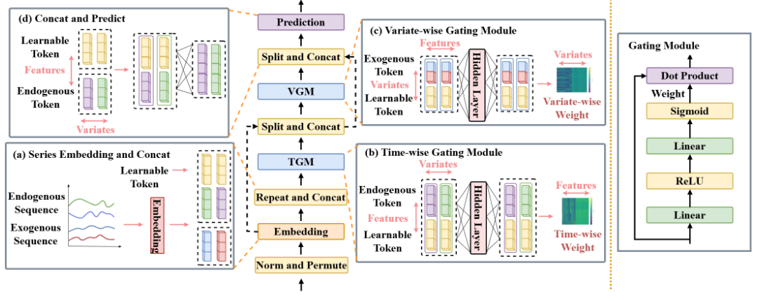
Here, the main addition comes from the gating mechanisms: time-wise gating and variate-wise gating. With these in place, the model can leverage informative signal from features through cross-variable dependencies and global tokens are derived from the input series.

Of course, there is much more to uncover, so let’s go through each element in more detail.

Embedding

The first key element of XLinear is its embedding layer as shown below.

 There, the input time series is first scaled using RevIN. Then, the embedding layer is learned. 

Notice that both exogenous and endogenous features are embedded within the same layer. Also, a global context token is introduced to bridge information between the series and the features.

Time-wise Gating Module (TGM)

Then, we enter the time-wise gating module (TGM) where the model learns temporal patterns from the input series.

Here, an MLP captures time dependencies and maps the input series to the global token. This is then used as time-wise gating weights fed through a sigmoid function for feature filtering.

Variate-wise Gating Module (VGM)

The next step is the variate-wise gating module as shown below.

Having learned temporal patterns from the target series, the model now learns associations between the features and the series. 

This is done by taking the global tokens from the previous step and learning the relationship between them and the exogenous sequences.

Prediction head

The final step is of course the prediction head.

There, a fully connected layer directly maps the learned tokens to the target sequence. 

At this point, the tokens contain information from temporal dependencies and cross-variate dependencies. They are all combined and passed through an MLP to jointly predict all target series.

As such, XLinear is a multivariate model where each target series acts as an endogenous target and an exogenous feature. However, in practice, we can specify if a series should be treated as an exogenous sequence only.

Thus, we can see how XLinear adapts the TimeXer model to use MLPs across each step, ensuring the model stays fast, lightweight, while still leveraging information from exogenous features.

Now that we have a deeper understanding of the inner workings of XLinear, let’s see it in action.

Forecasting with XLinear

To work with XLinear, I strongly suggest the use of neuralforecast, as this is the only library where the model is implemented on top of a user-friendly API.

Note that at the time of writing this article, XLinear is not part of the latest release of neuralforecast just yet. You might need to install neuralforecast from the main branch to access the model. 

For this little experiment, we will try to reproduce the results achieved by XLinear on the ETTm1 dataset. Specifically, we consider the multivariate case on a horizon of 96 time steps.

The ETTm1 dataset is part of the Electricity Transformer dataset which tracks the load and oil temperature of two electricity transformers in China. It is a very popular benchmark dataset in the time series forecasting literature, and it is released under the Creative Commons Attribution license.

The source code to reproduce this section is on GitHub.

Let’s get started!

Initial setup

First, we import the required packages for this experiment.

import pandas as pd

from datasetsforecast.long_horizon import LongHorizon

from neuralforecast.core import NeuralForecast
from neuralforecast.models import XLinear

from utilsforecast.losses import mae, mse
from utilsforecast.evaluation import evaluate

Again, we leverage neuralforecast to access XLinear, while giving us access to many more deep learning models. 

Also notice that we use datasetsforecast to load the data from ETTm1 directly in the format expected by neuralforecast.

Then, we create a function to help us load the different parts of the Electricity Transformer dataset.

def load_data(name):
    if name == "ettm1":
        Y_df, exog_df, static_df = LongHorizon.load(directory='./', group='ETTm1')
        Y_df['ds'] = pd.to_datetime(Y_df['ds'])
        val_size = 11520
        test_size = 11520
        freq = '15T'
    elif name == "ettm2":
        Y_df, *_ = LongHorizon.load(directory='./', group='ETTm2')
        Y_df['ds'] = pd.to_datetime(Y_df['ds'])
        val_size = 11520
        test_size = 11520
        freq = '15T'
    elif name == 'etth1':
        Y_df, exog_df, static_df = LongHorizon.load(directory='./', group='ETTh1')
        Y_df['ds'] = pd.to_datetime(Y_df['ds'])
        val_size = 2880
        test_size = 2880
        freq = 'H'
    elif name == "etth2":
        Y_df, *_ = LongHorizon.load(directory='./', group='ETTh2')
        Y_df['ds'] = pd.to_datetime(Y_df['ds'])
        val_size = 2880
        test_size = 2880
        freq = 'H'

    return Y_df, val_size, test_size, freq, exog_df, static_df

Here, we will focus on the ETTm1 dataset, but feel free to use any other portion of the dataset.

Then, we can load the ETTm1 dataset and set the horizon with:

Y_df, val_size, test_size, freq, exog_df, _ = load_data('ettm1')
horizon = 96

Note that while we fetch the exogenous features of ETTm1, we will not use them here because we are focusing on the multivariate case. This means that each series (there are 7 series in the dataset) will be both targets and exogenous features for each other.

Training and predicting with XLinear

Then, we can initialize XLinear. Here, we use the exact same hyperparameters as used by the researchers.

models = [
    XLinear(
        h=horizon, 
        input_size=horizon, 
        n_series=7,
        hidden_size=512,
        temporal_ff=256,
        channel_ff=21,
        head_dropout=0.5,
        embed_dropout=0.2,
        learning_rate=1e-4,
        batch_size=32,
        max_steps=2000, 
        early_stop_patience_steps=3),
]

There are few things to note before moving on:

1. Since XLinear is a multivariate model, neuralforecast requires us to define the number of series to predict. In this case, there are seven series, so n_series=7 .
2. The parameter channel_ff represents the dimension of the cross-channel feedforward layer in the variate-wise gating block. While you can technically use any arbitrary value, it is recommended to use a multiple of n_seriesfor better cross-channel modeling. Here, the researchers set it to 21.

Next, we can create an instance of the NeuralForecast object to handle model fitting and predictions.

nf = NeuralForecast(models=models, freq=freq)

Now, we can run cross-validation to effectively recreate the same modeling procedure as in the original paper.

nf_preds = nf.cross_validation(df=Y_df, val_size=val_size, test_size=test_size, n_windows=None)
nf_preds = nf_preds.reset_index()

Evaluation

Once the model is done training and predictions are obtained across the test set, we can evaluate the model using utilsforecast.

Here, we use both the MAE and MSE to evaluate the performance of XLinear, and we average the metrics across all seven targets.

ettm1_evaluation = evaluate(df=nf_preds, metrics=[mae, mse], models=['XLinear'], agg_fn="mean")

The results are shown in the table below:

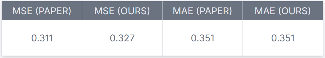
From the table above, we can see that we achieve the exact same MAE as reported by the authors of XLinear. For the MSE, we are off by only 5%, but we can still safely conclude that the implementation is neuralforecast is sound.

Thus, we can see how we can easily use XLinear in multivariate scenario. The model can also be used with all types of exogenous features:

• covariate with known future values through the futr_exog_list parameter
• covariates with only known values in the past through the hist_exog_list 
• static features that do not change in time through the stat_exog_list

All of those parameters are documented in neuralforecast allowing you to adapt XLinear to your own use case.

Conclusion

XLinear adapts the transformer-based TimeXer model to use the simpler MLP architecture. This results in a lighter and faster model that still achieves better forecasting performances.

The different gating modules allow XLinear to learn both temporal patterns in the target series and cross-variate dependencies with exogenous features. Plus, with its multivariate capability, the model can consider the inter-dependency between multiple target series.

In our small experiment, we were able to reproduce the results from the original paper, demonstrating the implementation is correct and verifying the performance of XLinear.

As always, each problem requires its own solution, and now you can test if XLinear is now the best answer to your scenario.

Thanks for reading! I hope that you enjoyed it and that you learned something new!

Learn the latest time series analysis techniques with my free time series cheat sheet in Python! Get the implementation of statistical and deep learning techniques, all in Python and TensorFlow!

Cheers 🍻

Next steps

If you are looking to level up your forecasting skills, check out some of my courses:

• Applied Time Series Forecasting in Python — the shortcut mastering time series forecasting where I teach everything I learned about forecasting, from statistical models to machine learning and deep learning models.
• Foundation Models for Time Series — take TimeGPT, Chronos, TimesFM and more, and apply them for zero-shot forecasting, fine-tune them, and incorporate exogenous features for state-of-the-art results. 

References

[1] X. Chen, H. Jin, Y. Huang, and Z. Feng, “XLinear: A Lightweight and Accurate MLP-Based Model for Long-Term Time Series Forecasting with Exogenous Inputs,” arXiv.org, 2026. https://arxiv.org/abs/2601.09237.

‌