Conformal Prediction in Time Series Forecasting

Consider the task of forecasting call volumes in a call center. The predictions play a primordial role, as they inform the budget allocation and workforce planning (if more calls are expected, more agents should be available to answer).

So we build a forecasting model and report that next week the center will receive 2451 calls.

Of course, with any prediction in the future comes some error and uncertainty. But how can we quantify it?

The logical answer is using prediction intervals. That way, we can report a range of possible future values with a certain confidence level.

While there are many methods for calculating prediction intervals, they are not applicable for all models and often rely on a particular distribution. 

This comes with two major problems. First, the distribution assumption may not hold in certain scenarios. Second, we may be restricted in our choice of modeling techniques.

For example, there are no straightforward ways to measuring prediction intervals for neural networks, but these models can possibly generate better predictions.

This is where conformal predictions come in. They represent a method of quantifying uncertainty in predictions that is both model-free and distribution-free.

In this article, we first explore the general idea behind conformal predictions and discover the EnbPI method for time series forecasting. Finally, we apply it in a small forecasting exercise.

Learn the latest time series analysis techniques with my free time series cheat sheet in Python! Get the implementation of statistical and deep learning techniques, all in Python and TensorFlow!

Let’s get started!

Quick overview of conformal predictions

Conformal predictions represent an entire field of study to quantify uncertainty in predictions.

They are applied across various tasks like regression, binary classification, multilabel classification and time series forecasting.

The general idea behind conformal predictions is to generate a calibrated prediction interval, at a given confidence level, that guarantees that a point will lie inside it.

In other words, with conformal predictions, you can create an 80% confidence interval that guarantees that the future real value will fall inside that interval 80% of the time.

Unlike other methods of estimating predictions intervals, conformal predictions can be used with any modeling techniques. Plus, they do not assume a normal distribution, which is usually the case for statistical methods.

Conformal predictions for time series forecasting

Now, most methods of conformal predictions for regressions tasks rely on the exchangeability hypothesis. 

This means that the order in which data arrives does not impact inference.

While this holds true for many regression scenarios, it is obviously not applicable in the context of time series forecasting.

We know that time series are points ordered in time and that order must remain intact. In other words, Monday must always come after Sunday and before Tuesday.

Hence the need for a dedicated method for generating conformal prediction for time series.

In 2020, researchers Chen Xu and Yao Xie presented the Ensemble batch Prediction Intervals (EnbPI) method in their article Conformal prediction for time series. 

This method removes the data exchangeability requirement and can thus be applied in time series forecasting.

Explore the EnbPI method

The EnbPI algorithm is a general conformal prediction framework for time series.

At a high level, the EnbPI method is composed of a training phase and a prediction phase. The training phase is shown in blue, and the prediction phase is shown in green in the figure below.

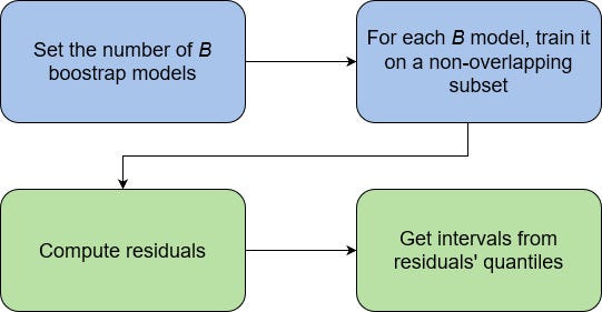
During the training phase, we fit a fixed number of B bootstrap models on non-overlapping subsets of the data. Usually, B is set to a value between 20 and 50.

Of course, the number of models that we can fit depends on the amount of data available, especially since the subsets cannot overlap.

Then, the predictions from each B model are aggregated in a leave-one-out (LOO) fashion, resulting in both LOO residuals and LOO models for predictions.

In the prediction phase, EnbPI uses each predictor to make a prediction on every single test data point. The predictions are aggregated to compute the center of the prediction interval. Then, using the residuals, prediction intervals are constructed using the quantiles from the residuals. The width is also optimized in the process, such that we get the narrowest width possible for a certain confidence level.

Note that in the prediction phase, as new values are observed, the intervals are updated to ensure their adpativeness.

Now that we understand how the EnbPI method can generate prediction intervals for any forecasting model, let’s apply it in a small forecasting project using Python.

Apply EnbPI in forecasting

We are now ready to use the EnbPI method to generate prediction intervals for our forecasting model.

Luckily for us, the EnbPI algorithm is implemented and ready to use through the MAPIE library, which stands for Model Agnostic Prediction Interval Estimator.

Here, we use a dataset recording the daily visits to a website’s blog, publicly available here.

As always, the entire source code for this project is available on GitHub.

The natural first step is to make the necessary imports and read our data.

import numpy as np
import pandas as pd
import matplotlib.pyplot as plt

from sklearn.ensemble import HistGradientBoostingRegressor

df = pd.read_csv('data/medium_views_published_holidays.csv')
df = df.drop(['unique_id'], axis=1)

df.head()

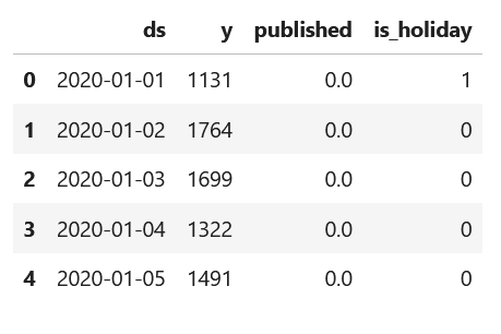
From the figure above, we see that our dataset contains a timestamp, the number of unique visitors, a flag to indicate if a new article was published or not, and a flag to indicate a national holiday.

Since we will be applying a machine learning model, we need to construct some features. Specifically, we extract the year, month and day from the date. We also add a flag to indicate the weekend and add the past seven lagged values.

df['ds'] = pd.to_datetime(df['ds'])

# Extract year, month and day
df['year'] = df['ds'].dt.year
df['month'] = df['ds'].dt.month
df['day'] = df['ds'].dt.day

# Add a flag for weekend days
df['is_weekend'] = (df['ds'].dt.dayofweek >= 5).astype(int)

# Add lagged values for the past 7 days
for day in range(1, 8):
    df[f'lag_{day}'] = df['y'].shift(day)

# Assign the date to the index
df.index = df['ds']
df = df.drop(['ds'], axis=1)

df.head()

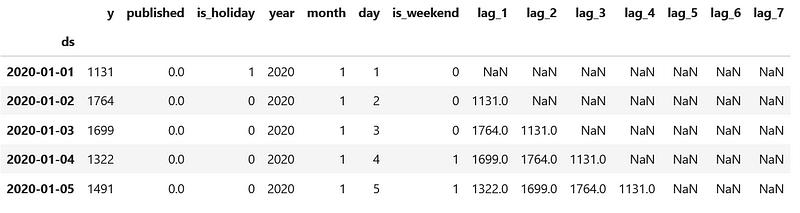
In the figure above, we notice that we have missing values. This is normal, since the first seven entries of the dataset do not have a complete list of seven past values.

We can either drop the first seven rows of data or use a model that can natively deal with missing data. In this case, I decided to use a Histogram-based Gradient Boosting Regressor, which natively supports data with missing values.

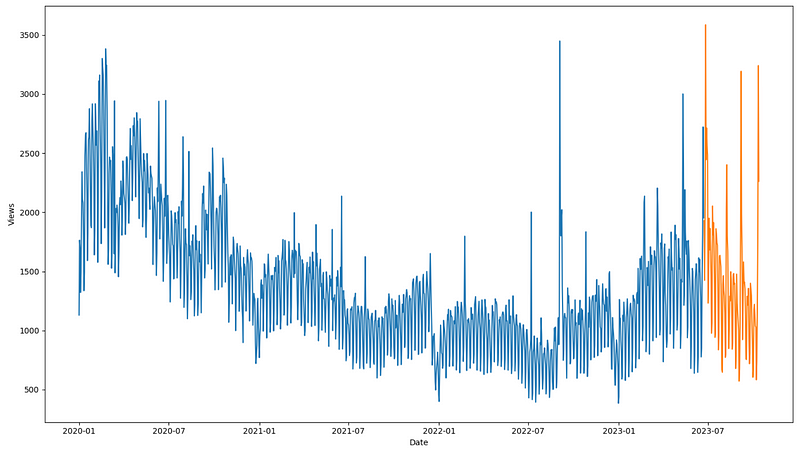
Finally, we split our data into a training and a test set. Here, I decided to reserve 112 time steps for the test set.

test_size = 4 * 28

X_cols = df.columns.drop(['y'])

split_date = df.index[-test_size]

X_train = df[df.index < split_date][X_cols]
y_train = df[df.index < split_date]['y']

X_test = df[df.index >= split_date][X_cols]
y_test = df[df.index >= split_date]['y']

print(X_train.shape, y_train.shape, X_test.shape, y_test.shape)

Optionally, we can visualize the split of our data resulting in the figure below.

fig, ax = plt.subplots(figsize=(14, 8))

ax.plot(y_train)
ax.plot(y_test)
ax.set_xlabel('Date')
ax.set_ylabel('Views')

plt.tight_layout()

Train a model

Once the data is preprocessed and split, we can focus on training a forecasting model.

As mentioned, we implement here a histogram-based gradient boosting regressor. We also perform hyperparameter tuning to have the optimal model using random search.

from sklearn.model_selection import RandomizedSearchCV, TimeSeriesSplit

hgbr = HistGradientBoostingRegressor(random_state=42)

params = {
    "learning_rate":  ["squared_error", "absolute_error", "gamma"],
    "learning_rate": [0.1, 0.05, 0.001],
    "max_iter": [100, 150, 200],
    "min_samples_leaf": [1, 2, 3],
}

rand_search_cv = RandomizedSearchCV(
    hgbr,
    param_distributions=params,
    cv=TimeSeriesSplit(n_splits=5),
    scoring="neg_root_mean_squared_error",
    random_state=42,
    n_jobs=-1
)

rand_search_cv.fit(X_train, y_train)

model = rand_search_cv.best_estimator_

Note that the best model is then saved using the best_estimator_ attribute.

Once we have an optimized model, we can now build prediction intervals using the EnbPI method. 

Estimate prediction intervals

First, we make the necessary imports for this step.

from mapie.metrics import regression_coverage_score, regression_mean_width_score
from mapie.subsample import BlockBootstrap
from mapie.regression import MapieTimeSeriesRegressor

To apply the EnbPI algorithm, we must use the MapieTimeSeriesRegressor object with BlockBootstrap. Remember that EnbPI fits a fixed number of models on non-overlapping blocks, and BlockBootstrap handles that for us.

Then, to evaluate the quality of our prediction intervals, we use the coverage and mean width score. Coverage reports the percentage of actual values that fall inside the intervals. The mean width score simply reports the average width of confidence intervals. 

In an ideal situation, we have the narrowest intervals possible achieving the highest coverage possible.

With all of that in mind, let’s complete the setup to generate the intervals. Here, we wish to have 95% confidence intervals, and our model will make forecasts for the next time step.

# For a 95% confidence interval, use alpha=0.05
alpha = 0.05

# Set the horizon to 1
h = 1

cv_mapie_ts = BlockBootstrap(
    n_resamplings=9,
    n_blocks=9,
    overlapping=False,
    random_state=42
)

mapie_enbpi = MapieTimeSeriesRegressor(
    model,
    method='enbpi',
    cv=cv_mapie_ts,
    agg_function='mean',
    n_jobs=-1
)

In the code block above, note that we use n_blocks=9 since the training set is divisible by 9. Also, make sure to set overlapping=False as the EnbPI methods requires the blocks to be non-overlapping.

Then, the regression model is simply wrapped in the MapieTimeSeriesRegressorobject, which we can then fit and use to make predictions.

mapie_enbpi = mapie_enbpi.fit(X_train, y_train)

y_pred, y_pred_int = mapie_enbpi.predict(
    X_test,
    alpha=alpha,
    ensemble=True,
    optimize_beta=True
)

Now, we have access to both the predictions of the model and the confidence intervals. We can visualize them using the code block below.

fig, ax = plt.subplots(figsize=(14, 8))

ax.plot(y_test, label='Actual')
ax.plot(y_test.index, y_pred, label='Predicted', ls='--')
ax.fill_between(
    y_test.index,
    y_pred_int[:, 0, 0],
    y_pred_int[:, 1, 0],
    color='green',
    alpha=0.2
)
ax.set_xlabel('Date')
ax.set_ylabel('Views')
ax.legend(loc='best')

plt.tight_layout()

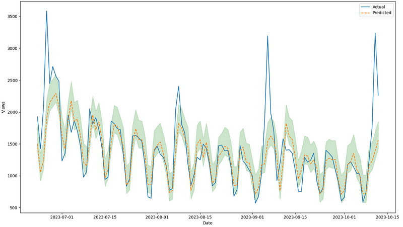
From the figure above, we can see that the model fails to predict the peaks in visitors. However, it seems that the prediction intervals contain the majority of the actual values.

To verify that, we can compute the coverage and mean interval width.

coverage = regression_coverage_score(
    y_test, y_pred_int[:, 0, 0], y_pred_int[:, 1, 0]
)
width_interval = regression_mean_width_score(
    y_pred_int[:, 0, 0], y_pred_int[:, 1, 0]
)

Here, we get a coverage of 58% and a mean interval width of 432. 

Again, in an ideal situation, the coverage should approach the value of 95%, since that was the probability that we set earlier. However, due to the model not being able to forecast those peaks, the coverage clearly suffered.

To potentially improve the coverage, let’s implement the EnbPI method with partial fit so that the intervals can adapt as new values are observed.

Apply EnbPI with partial fit

As we learned earlier, the EnbPI method can benefit from new observed values and tweak the confidence intervals accordingly. 

This can be simulated by fitting the model on parts of data and computing the prediction intervals at each step.

y_pred_pfit = np.zeros(y_pred.shape)
y_pred_int_pfit = np.zeros(y_pred_int.shape)

y_pred_pfit[:h], y_pred_int_pfit[:h, :, :] = mapie_enbpi.predict(X_test.iloc[:h, :],
                                                                 alpha=alpha,
                                                                 ensemble=True,
                                                                 optimize_beta=True)

for step in range(h, len(X_test), h):
    mapie_enbpi.partial_fit(X_test.iloc[(step-h): step, :],
                             y_test.iloc[(step-h):step])
    
    y_pred_pfit[step:step + h], y_pred_int_pfit[step:step + h, :, :] = mapie_enbpi.predict(X_test.iloc[step:(step+h), :],
                                                                                           alpha=alpha,
                                                                                           ensemble=True,
                                                                                           optimize_beta=True)

In the code block above, the logic remains identical. This time, we are simply doing a for loop to gradually fit the model on more data, simulating the fact that new data is being observed and generating a new prediction.

Again, we can visualize the predictions and their confidence intervals.

fig, ax = plt.subplots(figsize=(14, 8))

ax.plot(y_test, label='Actual')
ax.plot(y_test.index, y_pred_pfit, label='Predicted', ls='--')
ax.fill_between(
    y_test.index,
    y_pred_int_pfit[:, 0, 0],
    y_pred_int_pfit[:, 1, 0],
    color='green',
    alpha=0.2
)
ax.set_xlabel('Date')
ax.set_ylabel('Views')
ax.legend(loc='best')

plt.tight_layout()

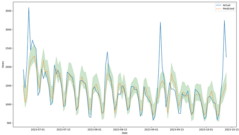
Visually, from the figure above, it seems that using partial fit does not make a significant difference.

For that reason, let’s compute the coverage and mean interval width for the partial fit protocol.

coverage_pfit = regression_coverage_score(
    y_test, y_pred_int_pfit[:, 0, 0], y_pred_int_pfit[:, 1, 0]
)
width_interval_pfit = regression_mean_width_score(
    y_pred_int_pfit[:, 0, 0], y_pred_int_pfit[:, 1, 0]
)

This gives us a coverage of 63% and an average interval width of 436.

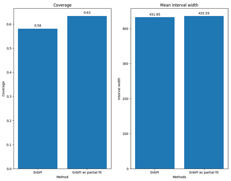
From the figure above, we can see that using partial fit allows us to increase the coverage while keeping the mean interval width fairly constant. Therefore, there is an advantage in using partial fit in this situation.

Conclusion

In this article we learned that conformal predictions group methodologies to estimate uncertainty in predictions. They can be applied for both classification and regression algorithms.

In the case of time series, the Ensemble Prediction Interval method fits a fixed number of models over non-overlapping blocks of data to get the residuals and estimate the confidence bounds from their distribution. 

To evaluate the quality of our intervals, we use the coverage and mean interval width. The coverage indicates the percentage of true values that fall inside the intervals. Ideally, this value should approach the confidence set by the user, while minimizing the width of the interval.

As we have seen, this is not always the case, as it also depends on the quality of the predictions of the model. 

Still, thanks to MAPIE, we can generate conformal prediction intervals for virtually any model.

Thanks for reading! I hope that you enjoyed it and that you learned something new!

Looking to master time series forecasting? Then check out my course Applied Time Series Forecasting in Python. This is the only course that uses Python to implement statistical, deep learning and state-of-the-art models in 16 guided hands-on projects.

Cheers 🍻

Support me

Enjoying my work? Show your support with Buy me a coffee, a simple way for you to encourage me, and I get to enjoy a cup of coffee! If you feel like it, just click the button below 👇

References

Chen Xu, Yao Xie — Conformal Predictions for Time Series

MAPIE: official documentation