Chronos: The Latest Time Series Forecasting Foundation Model by Amazon

The field of time series forecasting has been in effervescence lately, with a lot of work being done on foundation forecasting models.

It all started in October 2023 with the release of TimeGPT, one of the very first foundation model capable of zero-shot forecasting and anomaly detection.

Then, many efforts were done to adapt LLMs to forecasting tasks, like PromptCast and LLMTime. 

Following that, we saw more open-source foundation models, like Lag-LLaMA for probabilistic zero-shot forecasting and Time-LLM which reprograms existing off-the-shelf language models for time series forecasting. 

Now, in March 2024, the company Amazon has also entered the game with the release of Chronos.

In their paper, Chronos: Learning the Language of Time Series, the authors propose a framework for zero-shot probabilistic forecasting that leverages existing transformer-based language model architectures. It can minimally adapt existing language models for forecasting tasks.

In this article, we explore the inner workings of Chronos; how it was trained, and the data augmentation techniques used to pre-train large models. Then, we apply Chronos is our own small experiment, using Python, to see it in action.

For more details, make sure to read the original paper.

Learn the latest time series analysis techniques with my free time series cheat sheet in Python! Get the implementation of statistical and deep learning techniques, all in Python and TensorFlow!

Let’s get started!

Explore Chronos

The motivation behind Chronos started with the very naive question:

Shouldn’t good language models just work for time series forecasting?

This is not the first time that we try to adapt natural language processing (NLP) technologies to time series forecasting.

After all, in both fields, models attempt to learn a sequence of data to predict the next token, whether that token is a word or a real value.

However, in NLP, there are a fixed number of words to choose from, whereas in time series, it is technically unbounded; your series can increase or decrease indefinitely.

Therefore, directly using large language models (LLMs) for forecasting makes no sense, and they must be adapted for such task.

To that end, Chronos is a framework that adapts existing LLMs for time series forecasting. This framework allowed the researchers to pre-train a family of models for zero-shot forecasting.

Overview of Chronos

There are three main steps in Chronos to adapt LLMs for forecasting.

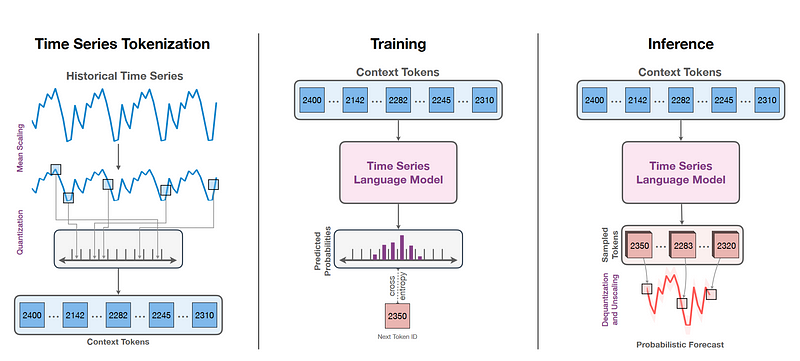
From the figure above, we can see that Chronos firsts scales the data and performs quantization before generating context tokens.

Then, these tokens can be used to train an existing language model that will predict the next context token. 

That prediction is then dequantized and unscaled to get the actual forecast.

Let’s take a look at each step in more detail.

Tokenization of time series

Since LLMs work with tokens of a finite vocabulary, we need to find a way to map time series values to a finite set of tokens. To that end, the authors propose to scale and then quantize the observations into a fixed number of bins.

There are many techniques for scaling data, such as min-max scaling, mean scaling and standard scaling. Here, the authors used mean scaling, which follows the simple formula:

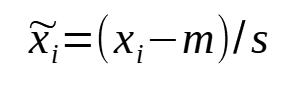
Where m is set to 0, and s is the mean of the absolute values of the series.

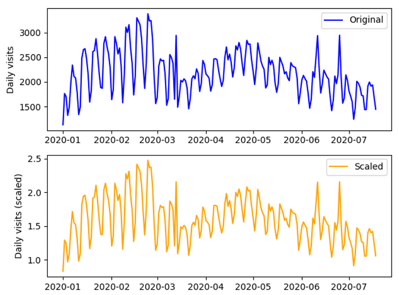
From the figure above, we can see that scaling our data keeps its shape in time, but we restrict the values to a smaller set. That way, it will be easier to represent these values as a fixed set of tokens to train the LLM.

Once the data is scaled, quantization is applied. This is a critical step, as the scaled series is still real-valued, and LLM cannot handle that type of data.

Quantization is a process that maps continuous infinite values to a set of discrete finite values. This is how we can create context tokens from time series data to feed the LLMs.

In the context of Chronos, the researchers use binning. This involves creating bins where the smallest value will pertain to the first bin, and the largest value of the series is assigned to the last bin. Then, each bin edge is uniformly spread out across the range of values in the series, and each value is assigned to a bin.

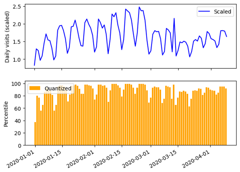
In the figure above, we can see an example of quantization using percentile binning. We define 100 bins, one for each percentile, and assign the scaled values to their corresponding bin. 

That way, we have now a series of fixed tokens, since with percentile binning, the token can only take values from 1 to 100. 

Thus, we have successfully tokenized a time series from infinite real values, to a fixed set of tokens, which is what is expected by LLMs.

Note that in Chronos, there is no encoding of common temporal features, like day-of-week, day-of-year, etc. Instead, Chronos considers the series as a simple sequence of tokens. 

This is surely counter-intuitive, but it allows minimal adaptation of the language model.

Training

Once the time series is tokenized, it can be sent to the LLM for training. Here, the authors use the categorical cross-entropy loss as the loss function for model training.

This means that the model learns to associate nearby bins together. In other words, they are learning a distribution.

This allows the model to learn arbitrary distributions and potentially better generalize on unseen data for zero-shot forecasting.

This is also unlike typical approaches. Usually, models force some kind of distribution for probabilistic forecasts, like the Gaussian or Student’s-t (the latter being used in Lag-LLaMA).

Inference

Once the model is trained, it can then perform forecasting.

We simply feed context tokens, which the model uses to generate a sequence of future tokens. 

Those tokens are then dequantized, which results in scaled predictions.

So, the transformation is reverse, which scales the data back to the original scale and we then have the final predictions.

Now that we understand how Chronos adapts LLMs for time series forecasting, there remains a big challenge to create performant foundation forecasting models: access to data.

To that end, the researchers propose two data augmentation methods: TSMix and KernelSynth.

Data augmentation

Foundation models rely on large and diverse datasets. While that is possible for natural language, time series data are not as accessible.

Therefore, the researchers used two data augmentation technique to increase and diversify their training set.

TSMix — Time Series Mixup

The first method is TSMix which stands for Time Series Mixup.

The idea behind TSMix is very simple. It will randomly sample subsequences of existing time series of a specific length, scale them, and take their convex combination.

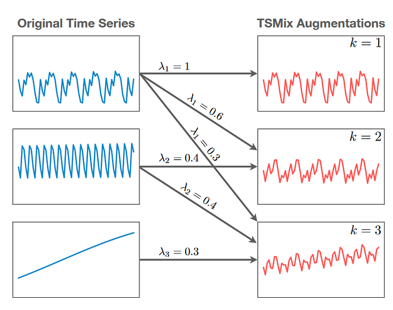
From the figure above, we can see how series as sampled and then combined with other series using different weights to generate another series for training.

KernelSynth

To further extend their training set, the authors also propose KernelSynth, a method to generate synthetic time series using Gaussian processes as shown below.

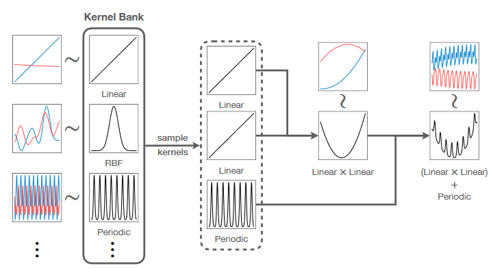
With KernelSynth, there is a bank of kernels defining a general behavior of time series: linear, periodic, etc.

In the figure above, we can see that the linear kernel is combined with itself using a multiplication, resulting in a quadratic shape. Then, that is combined again with the periodic kernel, using addition, adding a seasonal pattern.

From there, the kernel is fed to a Gaussian process, which takes care of generating samples within a certain distribution. 

Now that we understand how Chronos works and what data augmentation techniques were used to pre-train models, let’s actually use them in a small forecasting project using Python.

Forecasting with Chronos

Using the Chronos framework, the researchers already pre-trained five models that are publicly available for zero-shot forecasting.

The models were trained with the T5 architecture proposed by Google and are available at different sizes:

1. chronos-t5-tiny: 8M parameters
2. chronos-t5-mini: 20M parameters
3. chronos-t5-small: 46M parameters
4. chronos-t5-base: 200M parameters
5. chronos-t5-large: 710M parameters 

The weights of the models are all available on HuggingFace.

For this small experiment, we will use chronos-t5-large and test it on the M3 monthly dataset. It contains 1428 unique time series, all with a monthly frequency, from a variety of industries. It is publicly available here under the Creative Commons Attributes license.

We will also compare the performance of Chronos to that of MLP and N-BEATS. Note that M3 is a fairly small dataset and deep learning methods do not perform so well, but these models usually do well on small datasets.

As usual, the full code for this experiment is on GitHub.

Let’s get started!

Initial setup

First, we need to install Chronos to make use of it.

pip install git+https://github.com/amazon-science/chronos-forecasting.git

Then, let’s install the rest of the libraries for this experiment.

import time
from datasetsforecast.m3 import M3
import torch
from chronos import ChronosPipeline

Once this is done, we can load the dataset. Luckily for us, the library datasetsforecast gives us a Python interface to download the dataset.

Y_df, *_ = M3.load(directory='./', group='Monthly')

Great! Now, we can initialize Chronos. We instantiate a ChronosPipeline object and specify the pre-trained model that we want.

pipeline = ChronosPipeline.from_pretrained(
  "amazon/chronos-t5-large",
  device_map="cuda",
  torch_dtype=torch.bfloat16,
)

Now, we are ready to forecast!

Predicting with Chronos

For this experiment, we will loop through all available series in the M3 dataset and keep the last 12 values as a test set to evaluate the predictions.

Here, Chronos expects a torch.tensor as input, so we have to convert our pandas.Series to a numpy.array and then as a tensor.

All values before our test set will be fed to the model as context tokens.

Then, we simply call the predict method of our pipeline.

To get the actual predictions, we need to specify which quantile we are interested in, since Chronos generates probabilistic forecasts. In this case, we are interested only in the median value. However, for an 80% confidence interval, you could the pass the following list of percentiles: [0.1, 0.5, 0.9]. Make sure to always include quantile 0.5, as this represents the median value.

horizon = 12
batch_size = 12


actual = []
chronos_large_preds = []

start = time.time()
all_timeseries = [
    torch.tensor(sub_df["y"].values[:-horizon])
    for _, sub_df in Y_df.groupby("unique_id")
]
for i in tqdm(range(0, len(all_timeseries), batch_size)):
    batch_context = all_timeseries[i : i + batch_size]
    forecast = pipeline.predict(batch_context, horizon)
    predictions = np.quantile(forecast.numpy(), 0.5, axis=1)

    chronos_large_preds.append(predictions)

chronos_large_preds = np.concatenate(chronos_large_preds)
chronos_large_duration = time.time() - start
print(chronos_large_duration)

Alright! At this point, we have predictions from Chronos. Let’s then compare its performance with other models, such as an MLP and N-BEATS.

Forecasting with MLP and N-BEATS

Now, let’s train an MLP model and N-BEATS. Here, we keep the default configuration and use an input size of three times the horizon.

from neuralforecast.models import MLP, NBEATS
from neuralforecast.losses.pytorch import HuberLoss
from neuralforecast.core import NeuralForecast

horizon = 12
val_size = 12
test_size = 12

# Fit an MLP
mlp = MLP(h=horizon, input_size=3*horizon, loss=HuberLoss())

nf = NeuralForecast(models=[mlp], freq='M')
mlp_forecasts_df = nf.cross_validation(df=Y_df, val_size=val_size, test_size=test_size, n_windows=None, verbose=True)

# Fit N-BEATS
nbeats = NBEATS(h=horizon, input_size=3*horizon, loss=HuberLoss())

nf = NeuralForecast(models=[nbeats], freq='M')
nbeats_forecasts_df = nf.cross_validation(df=Y_df, val_size=val_size, test_size=test_size, n_windows=None, verbose=True)

Now that we have predictions from all of our models, let’s evaluate their performance.

Evaluation

First, let’s visualize the predictions of each model against the actual values.

fig, axes = plt.subplots(nrows=2, ncols=2, figsize=(14,12))

for i, ax in enumerate(axes.flatten()):
    id = f"M{i+1}"
    mlp_to_plot = mlp_forecasts_df[mlp_forecasts_df['unique_id'] == id]
    nbeats_to_plot = nbeats_forecasts_df[nbeats_forecasts_df['unique_id'] == id]

    ax.plot(mlp_to_plot['ds'], mlp_to_plot['y'], label='actual')
    ax.plot(mlp_to_plot['ds'], mlp_to_plot['MLP'], ls='--', label='MLP')
    ax.plot(nbeats_to_plot['ds'], nbeats_to_plot['NBEATS'], ls=':', label='N-BEATS')
    ax.plot(nbeats_to_plot['ds'], preds[0+12*i:12+12*i], ls='-.', label='Chronos')

    ax.legend()

In the figure above, we can see the predictions from each model of the first four series of our dataset. Again, we see that deep learning models struggle when the dataset is small.

Still, since Chronos is a deep learning model, I wanted to keep the comparison in the realm of deep learning.

Now, let’s compute the mean absolute error (MAE) and symmetric mean absolute percentage error (sMAPE) for each model.

For that, we use the utilsforecast library, which comes with many functions commonly used in time series projects for model evaluation, plotting, and data preprocessing.

from utilsforecast.losses import mae, smape
from utilsforecast.evaluation import evaluate

forecast_df = mlp_forecasts_df
forecast_df["NBEATS"] = nbeats_forecasts_df["NBEATS"]
forecast_df["Chronos-Tiny"] = chronos_pred_df["chronos_tiny_pred"]
forecast_df["Chronos-Large"] = chronos_pred_df["chronos_large_pred"]

evaluation = evaluate(
    forecast_df,
    metrics=[mae, smape],
    models=["MLP", "NBEATS", "Chronos-Tiny", "Chronos-Large"],
    target_col="y",
)

time = pd.DataFrame(
    {
        "metric": ["Time"],
        "MLP": [mlp_duration],
        "NBEATS": [nbeats_duration],
        "Chronos-Tiny": [chronos_tiny_duration],
        "Chronos-Large": [chronos_large_duration],
    }
)
avg_metrics = (
    evaluation.drop(columns="unique_id").groupby("metric").mean().reset_index()
)
avg_metrics = pd.concat([avg_metrics, time]).reset_index(drop=True)

avg_metrics

In the table above, we can see that N-BEATS is the champion model, as it achieves the lowest MAE and sMAPE.

It is important to note that N-BEATS and MLP achieve better performances than Chronos at a fraction of the time.

For this experiment, chronos-large took almost three times the time to perform zero-shot forecasting on the M3 dataset, compared to fitting and predicting with N-BEATS. On the other hand, chronos-tiny does achieve faster inference time, but it comes at the cost of lower performance.

Also, keep in mind that this experiment is highly influenced by my limited access to computation power.

We could make this experiment more robust by:

• Fine-tuning the MLP and N-BEATS model
• Using more datasets

For a more comprehensive benchmark of Chronos, see here.

My opinion on Chronos

Having testes Lag-LLaMA and Time-LLM in previous experiments, I can say that Chronos is much easier and faster to use.

I believe the researchers have done a great job at creating a foundation model that is actually usable. Although my experiment took 20 minutes to run, it is still much faster than Lag-LLaMA and Time-LLM.

However, we still do not have a foundation model that performs consistently better than data-specific models. 

Although foundation models allow for zero-shot forecasting, which technically simplifies the forecasting pipeline, they require a lot of computation power, take a lot of time to run, and ultimately do not perform than simple models.

I am curious to see how using the Chronos framework with another LLM would impact the performance of pre-trained models. 

Foundation forecasting models are still in early development, but for me, data-specific models still win.

Conclusion

Chronos is a framework to minimally adapt LLMs for time series forecasting. Using simple scaling and quantization methods, LLMs can be trained to perform forecasting tasks.

Researchers at Amazon used that framework to pre-train a family of zero-shot forecasters using the T5 architecture.

Those models can be used right away for zero-shot forecasting but keep in mind that they do take a lot of time to generate forecasts.

As always, I think that each problem requires its unique solution. Make sure to test Chronos against other methods.

Thanks for reading! I hope that you enjoyed it and that you learned something new!

Cheers 🍻

Learn the latest time series analysis techniques with my free time series cheat sheet in Python! Get the implementation of statistical and deep learning techniques, all in Python and TensorFlow!

Support me

Enjoying my work? Show your support with Buy me a coffee, a simple way for you to encourage me, and I get to enjoy a cup of coffee! If you feel like it, just click the button below 👇

References

Chronos: Learning the Language of Time Series by A. Ansari, L. Stella, C. Turkmen, X. Zhang, P. Mercado, H. Shen, O. Shchur, S. Rangapuram, S. Arango, S. Kapoor, J. Zschiegner, D. Maddix, M. Mahoney, K. Torkkola, A. Wilson, M. Bolhlke-Schneider, Y. Wang

Official repository of Chronos — GitHub