Catch Up on Large Language Models

If you are here, it means that like me you were overwhelmed by the constant flow of information, and hype posts surrounding large language models (LLMs). 

This article is my attempt at helping you catch up on the subject of large language models without the hype. After all, it is a transformative technology, and I believe it is important for us to understand it, hopefully making you curious to learn even more and build something with it.

In the following sections, we will define what LLMs are and how they work, of course covering the Transformer architecture. We also explore the different methods of training LLMs and conclude the article with a hands-on project where we use Flan-T5 for sentiment analysis using Python.

Let’s get started!

LLMs and generative AI: are they the same thing?

Generative AI is a subset of machine learning that focuses on models who’s primary function is to generate something: text, images, video, code, etc.

Generative models train on enormous amounts of data created by humans to learn patterns and structure which allow them to create new data.

Examples of generative models include:

• Image generation: DALL-E, Midjourney
• Code generation: OpenAI Codex
• Text generation: GPT-3, Flan-T5, LLaMA

Large language models are part of the generative AI landscape, since they take an input text and repeatedly predict the next word until the output is complete.

However, as language models grew larger, they were able to perform other tasks in natural language processing, like summarization, sentiment analysis, named entity recognition, translation and more.

With that in mind, let’s now focus our attention on how LLMs work.

How LLMs work

One of the reasons why we now have large language models is because of the seminal work of Google and University of Toronto when they released the paper Attention Is All You Need in 2017. 

This paper introduced the Transformer architecture, which is behind the LLMs we know and use today. 

This architecture unlocked large scale models, making it possible to train very large models on multiple GPUs, and the models are able to process the inputs in parallel, giving them the opportunity to treat very large sequences of data.

Overview of the Transformer architecture

The following is meant to be a high-level overview of the Transformer architecture. There are many resources that dive deeper into it, but the goal here is just to understand the way it works so we can understand how different LLMs specialize in different tasks.

At any time, for more details, I suggest you read the original paper.

So, let’s start with a simplified visualization of the Transformer architecture.

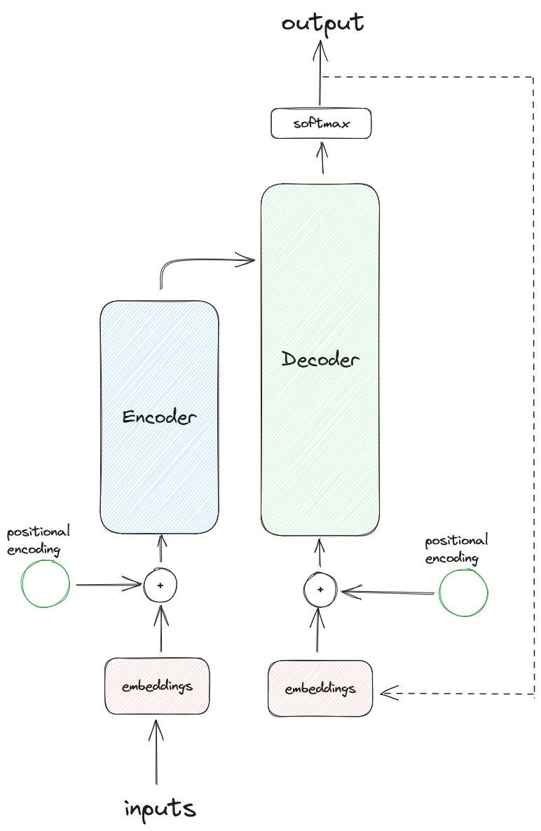
From the figure above, we can see that the main components of the Transformer are the encoder and decoder. Inside each, we also find the attention component.

Let’s explore each component in more detail to understand how the Transformer architecture works.

Tokenize the inputs

We know LLMs work with text, but computers work with numbers, not letters. Therefore, the input must be tokenized.

Tokenization is the process in which words of a sentence are represented as numbers. 

Basically, every possible word a model can work with is in a dictionary with a number associated to it. With tokenization, we can retrieve the number associated with the word, to represent a sentence as a sequence of numbers, as shown below.

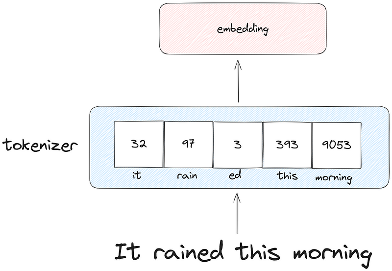
In the figure above, we see an example of how the sentence “It rained this morning” can be tokenized before being set to the embedding layer of the Transformer.

Note that there are many ways of tokenizing a sentence. In the example above, the tokenizer can represents parts of a word, which is why rained is separated into rain and ed. Other tokenizers would have a number for full words only.

The word embedding layer

At this point, we have a series of numbers that represent words, but how can the computer understand their meaning?

This is achieved by the word embedding layers.

Word embedding is a learned representation of words, such that words with a similar meaning will have a similar representation. The model will learn different properties of words and represent them in a fixed space, where each axis can represent the property of a word.

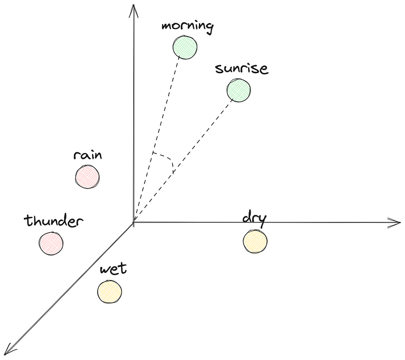
In the figure above, we can see how a 3D word embedding can look like. We see that “morning” and “sunrise” are closer to one another, and therefore have a similar representation. This can be can be computed using cosine similarity.

On the other hand, “rain” and “thunder” are close to each other, and far from “morning” and “sunrise”. 

Now, we can only show a 3D space, but in reality, embeddings can have hundreds of dimensions. In fact, the original Transformer architecture used an embedding space of 512 dimensions. This means that the model could learn 512 different properties of words to represent them in a space of 512 dimensions.

What about word order?

You may have noticed that by representing words in embeddings, we lose their order in the sentence. 

Of course, with natural language, word order is very important, and so that’s why we use positional encoding, so the model knows the order of the words in a sentence.

It is the combination of the word embeddings and the positional encoding that gets sent to the encoder.

Inside the encoder

Our inputs travel inside the encoder where they will go through the self-attention mechanism.

This is where the model can learn the dependencies between each token in a sentence. It learns the importance of each word in relation to all other words in a sentence. 

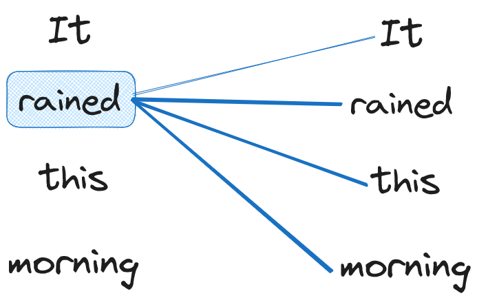
In the figure above, we have a stylized example of an attention map for the word “rained”. The stroke width represents the importance. 

In this example, we can see that self-attention captures the importance of “rained” with “this” and “morning”, meaning that it understands the context of this sentence.

While this example remains simple, since we have a very short sentence, the self-attention mechanism works very well on longer sentences, effectively capturing context and the overall meaning of a sentence.

Furthermore, the model does not have a single attention head. In fact, it has multiple attention heads, also called multi-headed self-attention, where each head can learn a different aspect of language. 

For example, in the paper Attention Is All You Need, the authors found that one head was involved in anaphora resolution, which is identifying the link between an entity and its repeated references.

Above, we see an example of anaphora resolution, where the word “keys” is later referenced as “they”, and so one attention head can specialize in identifying those links.

Note that we do not decide what aspect of language each attention head will learn. 

At this point, the model has a deep representation of the structure of meaning of a sentence. This is sent to the decoder.

Inside the decoder

The decoder accepts a deep representation of the input tokens. This informs the self-attention mechanism inside the decoder.

As a reminder, here is the Transformer architecture again, so we can remember what it looks like.

A start-of-sequence token is inserted as an input of the decoder, to signal it to start generating new tokens.

New tokens are generated according to the understanding of the input sequence generated by the encoder and its self-attention mechanism.

In the figure above, we can see that the output of the decoder gets sent to a softmax layer. This generates a vector of probabilities for each possible token. The one with the largest probability is then output by the model.

That output token is then sent back to the embeddings as an input to the decoder, until an end-of-sequence token is generated by the model. At that point, the output sequence is complete.

This concludes the basic architecture behind large language models. With the Transformer architecture and its ability to process data in parallel, it was possible to train models on huge amounts of data, making LLMs a reality. 

Now, there is more to this, as LLMs do not all use the full Transformer architecture, and that influences the way they are trained. Let’s explore this in more detail.

How LLMs are trained

We have seen the underlying mechanisms that power large language models, and as mentioned, not all models use the full Transformer architecture.

In fact, some models may use the encoder portion only, while others use the decoder portion only.

This means that the models are also trained differently and will therefore specialize in particular tasks.

Encoder-only models

Encoder-only models, also called autoencoding models are best suited for tasks like sentiment analysis, named entity recognition, and word classification

Popular examples of autoencoding models are BERT and ROBERTA.

Those models are trained using masked language modeling (MLM). With that training method, words in an input sentence are randomly masked, and the objective of the model is then to reconstruct the original text.

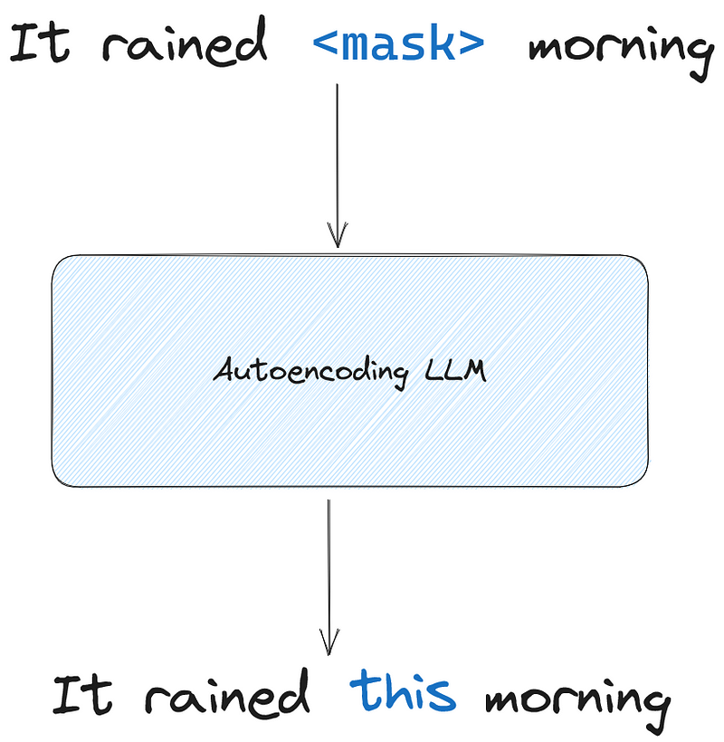
In the figure above, we can see what masked language modeling looks like. A word is hidden and the sentence is fed to the model, which must then learn to predict the right word to get the correct original sentence.

With that method, autoencoding models develop bidrectional context, since they see what precedes and follows the token they must predict, and not just what comes before.

Again, in the figure above, the model sees “it rained” and “morning”, so it sees both the beginning and the end of the sentence, allowing it to predict the word “this” to reconstruct the sentence correctly.

Note that with autoencoding models, the input and output sequences have the same length.

Decoder-only models

Decoder-only models are also called autoregressive models. These models are best suited for text generation, but new functions arise when the models get very large.

Example of autoregressive models are GPT and BLOOM.

These models are trained using causal language modeling (CLM). With causal language modeling, the model only sees the tokens preceding the mask, meaning that it does not see the end of the sequence.

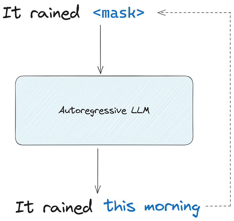
As we see above, with causal language modeling, the model only sees the tokens leading to the mask, and not what comes after. Then, it must predict the next tokens until the sentence is complete.

In the example above, the model would output “this”, and that token would be fed back as an input, so the model can then predict “morning”.

Unlike masked language modeling, model build unidirectional context, since they do not see what comes after the mask.

Of course, with decoder-only models, the output sequence can have a different length than the input sequence.

Encoder-decoder models

Encoder-decoder models are also called sequence-to-sequence models, and they use the full Transformer architecture.

Those models are often used for translation, text summarization and question answering.

Popular examples of sequence-to-sequence models are T5 and BART.

To train these models, the span corruption method is used. Here, a random sequence of tokens is masked and designated as a sentinel token. Then, the model must reconstruct the masked sequence autoregressively.

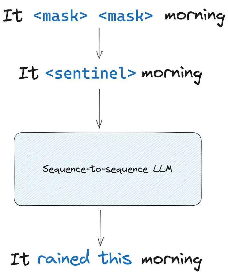
In the figure above, we can see that a sequence of two tokens were masked and replaced by a sentinel token. The model is then trained to reconstruct the sentinel token to obtain the original sentence.

Here, the masked input is sent to the encoder, and the decoder is responsible for reconstructing the masked sequence.

A note on model size

While we have specified certain tasks for which certain models perform best, researchers have observed that large models are capable of various tasks.

Therefore, very large decoder-only models can be very good at translation, even though encoder-decoder models specialize in that task.

With all of that in mind, let’s now start working with a large language in Python.

Work with a large language model

Before we get hands-on experience with a large language model, let’s just cover some technical terms involved when working with LLMs.

First, the text that we feed the LLM is called prompt, and the output of the model is called completion.

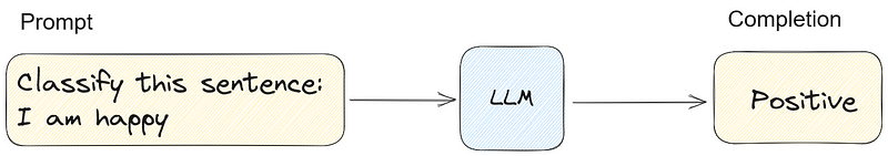
Inside the prompt is where we give the instructions to the LLM to achieve the task that we want.

This is also where prompt engineering is performed. With prompt engineering, we can perform in-context learning, which is when we give examples to the model of how certain tasks should be performed. We will see an example of that later on.

For now, let’s interact with an LLM using Python for sentiment analysis.

Hands-on project: sentiment analysis with Flan-T5

For this mini project, we use Flan-T5 for sentiment analysis of various financial news.

Flan-T5 is an improved version of the T5 model, which is a sequence-to-sequence model. Researchers basically took the T5 model and fine-tuned it on different tasks covering more languages. For more details, you can refer to the original paper.

As for the dataset, we will use the financial_phrasebank dataset published by Pekka Malo and Ankur Sinha under the Creative Commons Attribute license. 

The dataset contains a total of 4840 sentences from English language financial news that were categorized as positive, negative or neutral. A group of five to eight annotators classified each sentence, and depending on the agreement rate, the size of the dataset will vary (4850 rows for a 50% agreement rate, and 2260 rows for a 100% agreement rate).

For more information on the dataset and how it was compiled, refer to the full dataset details page.

Of course, all code show below is available on GitHub.

Setup your environment

For the following experiment to work, make sure to have a virtual environment with the following packages installed:

• torch
• torchdata
• transformers
• datasets
• pandas
• matplotlib
• scikit-learn

Note that the libraries transformers and datasets are from HuggingFace, making it super easy for us to access and experiment with LLMs.

Once the environment is setup, we can start by importing the required libraries.

import pandas as pd
import numpy as np
import matplotlib.pyplot as plt

from datasets import load_dataset
from transformers import AutoModelForSeq2SeqLM, AutoTokenizer, GenerationConfig

Load the data

Then, we can load our dataset. Here, we use the dataset with 100% agreement rate.

dataset_name = "financial_phrasebank"

dataset = load_dataset(dataset_name, "sentences_allagree")

This dataset contains a total of 2264 sentences.

Note that the label is encoded. 1 means neutral, 0 means negative and 2 means positive. The count of each label is shown below.

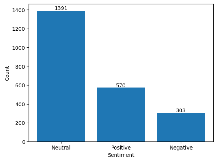
Let’s store the actual label of each sentence in a DataFrame, making it easier for us to evaluate the model later on.

labels_df = pd.DataFrame()

labels_from_dataset = [dataset['train'][i]['label'] for i in range(2264)]

labels_df['labels'] = labels_from_dataset

Load the model

Now, let’s load the model as well as the tokenizer. As mentioned above, we will load the Flan-T5 model. Note that the model is available in different sizes, but I decided to use the base version.

model_name = "google/flan-t5-base"

model = AutoModelForSeq2SeqLM.from_pretrained(model_name)

tokenizer = AutoTokenizer.from_pretrained(model_name, use_fast=True)

That’s it! We can now use this LLM to perform sentiment analysis on our dataset.

Prompt the model for sentiment analysis

For the model to perform sentiment analysis, we need to do prompt engineering to specify that task.

In this case we simply use “Is the following sentence positive, negative or neutral?”. We then pass the sentence of our dataset and let the model infer.

Note that this is called zero-shot inference, since the model was not specifically trained for this particular task on this specific dataset.

zero_shot_sentiment = []

for i in range(2264):
    sentence = dataset['train'][i]['sentence']

    prompt = f"""
Is the follwing sentence positive, negative or neutral?

{sentence}
    """

    inputs = tokenizer(prompt, return_tensors='pt')
    output = tokenizer.decode(
        model.generate(
            inputs["input_ids"],
            max_new_tokens=50
        )[0],
        skip_special_tokens=True
    )

    zero_shot_sentiment.append(output)

In the Python code block above, we loop over each sentence in the dataset and pass it in our prompt. The prompt is tokenized and set to the model. We then decode the output to obtain a natural language response. Finally, we store the prediction of the model in a list.

Then, let’s add these predictions to our DataFrame.

labels_df['zero_shot_sentiment'] = zero_shot_sentiment
labels_df['zero_shot_sentiment'] = labels_df['zero_shot_sentiment'].map({'neutral':1, 'positive':2, 'negative':0})

Evaluate the model

To evaluate our model, let’s display the confusion matrix of the predictions, as well as the classification report.

from sklearn.metrics import confusion_matrix, ConfusionMatrixDisplay
from sklearn.metrics import classification_report

cm = confusion_matrix(labels_df['labels'], labels_df['zero_shot_sentiment'], labels=[0,1,2])

disp_cm = ConfusionMatrixDisplay(cm, display_labels=[0,1,2])

disp_cm.plot();

plt.grid(False)
plt.tight_layout()


clf_report = classification_report(labels_df['labels'], labels_df['zero_shot_sentiment'], labels=[0,1,2])

print(clf_report)

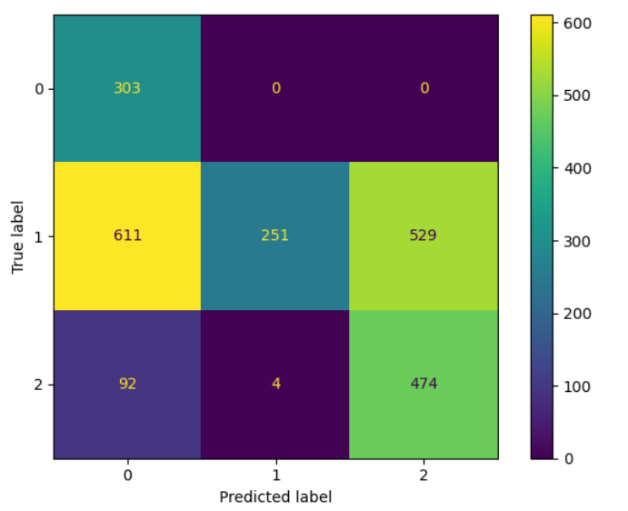
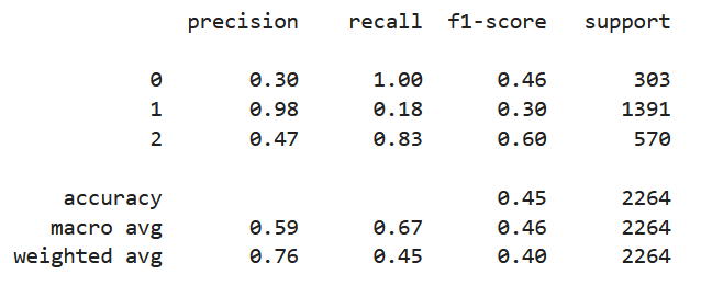
From the figure above, we can see that the model found all negative sentences, at the cost of precision since it mislabelled 611 neutral sentences and 92 positive sentences. Also, we can see a clear problem with identifying neutral sentences, as it mislabelled the vast majority.

Therefore, let’s try to change our prompt to see if we can improve the model’s performance.

One-shot inference with in-context learning

Here, we modify our prompt to include an example of a neutral sentence. This technique is called in-context learning, as we pass an example of how the model should behave inside the prompt.

Passing one example is called one-shot inference. It is possible to pass more examples, in which case it becomes few-shot inference. 

It is normal to show up to five examples to the LLM. If the performance does not improve, then it is likely that we need to fine-tune the model.

For now, let’s see how one example impacts the performance.

one_shot_sentiment = []

for i in range(2264):
    sentence = dataset['train'][i]['sentence']

    prompt = f"""

Is the follwing sentence positive, negative or neutral?

Statement: "According to Gran , the company has no plans to move all production to Russia , although that is where the company is growing ."
neutral

Is the follwing sentence positive, negative or neutral?
Statement: {sentence}

{sentence}
    """

    inputs = tokenizer(prompt, return_tensors='pt')
    output = tokenizer.decode(
        model.generate(
            inputs["input_ids"],
            max_new_tokens=50
        )[0],
        skip_special_tokens=True
    )

    one_shot_sentiment.append(output)

In the code block above, we see that we give an example of a neutral sentence to help the model identify them. Then, we pass each sentence for the model to classify.

Afterwards, we follow the same steps of adding a new columns containing the new predictions, and displaying the confusion matrix.

labels_df['one_shot_sentiment'] = one_shot_sentiment
labels_df['one_shot_sentiment'] = labels_df['one_shot_sentiment'].map({'neutral':1, 'positive':2, 'negative':0})

cm = confusion_matrix(labels_df['labels'], labels_df['one_shot_sentiment'], labels=[0,1,2])

disp_cm = ConfusionMatrixDisplay(cm, display_labels=[0,1,2])

disp_cm.plot();

plt.grid(False)
plt.tight_layout()

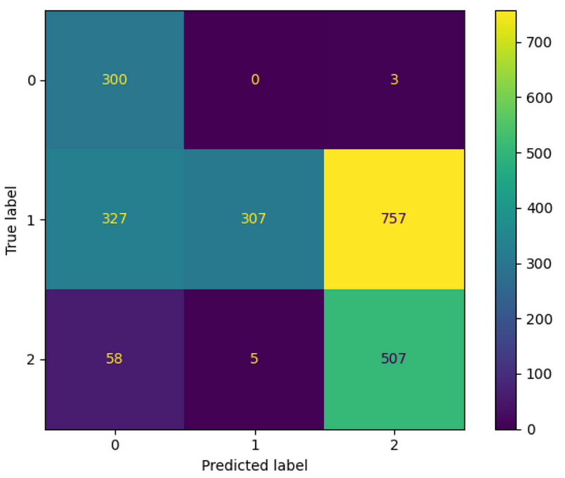
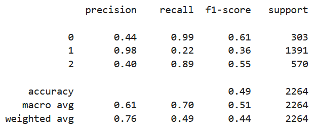
From the figure above, we can see a slight improvement. The weighted F1-score increased from 0.40 to 0.44. The model did better on the neutral class, but at the cost of a worse performance on the positive class.

Adding examples of positive, negative, and neutral sentences may help, but I did not test it out. Otherwise, fine-tuning the model would be necessary, but that is the subject of another article.

Conclusion

A lot of concepts were covered in this article, from the understanding the basics of LLMs, to actually using Flan-T5 for sentiment analysis in Python.

You now have the foundational knowledge to explore this world on your own and see how we can fine-tune LLMs, how we can train one, and how we can build applications around them.

I hope that you learned something new, and that you are curious to learn even more.

Cheers 🍻

Support me

Enjoying my work? Show your support with Buy me a coffee, a simple way for you to encourage me, and I get to enjoy a cup of coffee! If you feel like it, just click the button below 👇

References

Attention is All You Need — Ashish Vaswani, Noam Shazeer, Niki Parmar, Jakob Uszkoreit, Llion Jones, Aidan N. Gomez, Lukasz Kaiser, Illia Polosukhin

Generative AI with LLMs — deeplearning.ai