Basic Statistics for Time Series Analysis in Python

A time series is simply a set of data points ordered in time, where time is usually the independent variable.

Now, forecasting the future is not the only purpose of time series analysis. It is also relevant to asses important properties, such as stationarity, seasonality or autocorrelation.

Before moving on to more advanced modelling practices, we must master the basics first.

In this article, we will introduce the building blocks of time series analysis by introducing descriptive and inferential statistics. These concepts will serve later on when we implement complex models on time series, as statistical significance is necessary to build a robust analysis.

All code examples will be in Python and you can grab the notebook to follow along.

Let’s get started!

Use Python and TensorFlow to apply more complex models for time series analysis with my free time series cheat sheet!

Descriptive Statistics

Descriptive statistics are a set of values and coefficients that summarize a dataset. It provides information about central tendency and variability.

Values such as the mean, median, standard deviation, minimum and maximum are usually the ones we are looking for.

So, let’s see how we can obtain those values with Python.

First, we will import all of the required libraries. Not all of them are used for descriptive statistics, but we will use them later on.

import pandas as pd
import matplotlib.pyplot as plt
import matplotlib.mlab as mlab
import seaborn as sns

from sklearn.linear_model import LinearRegression

import statsmodels.api as sm

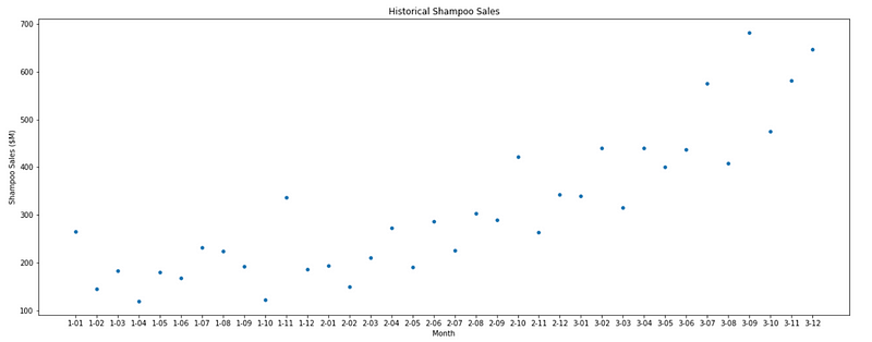
Now, we will explore the dataset shampoo.csv. This dataset traces the historical volume of sales of shampoo in a certain period of time.

In order to see the entire dataset, we can execute the following Python code:

data = pd.read_csv('shampoo.csv')
data

Be careful, as this will show the entire dataset. In this case, there are only 36 instances, but for larger datasets, this is not very practical.

Instead, we should use the following piece of code:

data.head()

The line of code above will show the first five entries of the dataset. You can decide to display more by specifying how many entries you would like to see.

data.head(10)

The line above will show the first 10 entries of a dataset.

Now, there is a very simple way to obtain the mean, median, standard deviation, and other information about the central tendency of the dataset.

Simply run the line of code below:

data.describe()

And you should see the following information for the shampoo dataset:

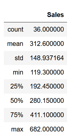
As you can see, with this simple method, we have information about the size of the dataset, its mean and standard deviation, minimum and maximum values, as well as information about its quartiles.

Visualizations

Numbers are a good starting point, but being able to visualize a time series can give you quick insights which will help you steer you analysis in the right direction.

Histograms and scatter plots are the most widely used visualizations when it comes to time series.

A simple histogram of our dataset can be displayed with:

data.hist()

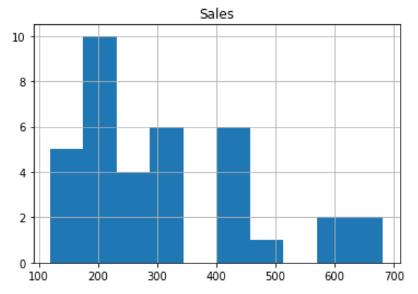
However, we can do much better. Let’s plot a better histogram and add labels to this axes.

plt.figure(figsize=[10, 7.5]); # Set dimensions for figure

plt.hist(data['Sales'])
plt.title('Histogram of Shampoo Sales');
plt.xlabel('Shampoo Sales ($M)');
plt.ylabel('Frequency');

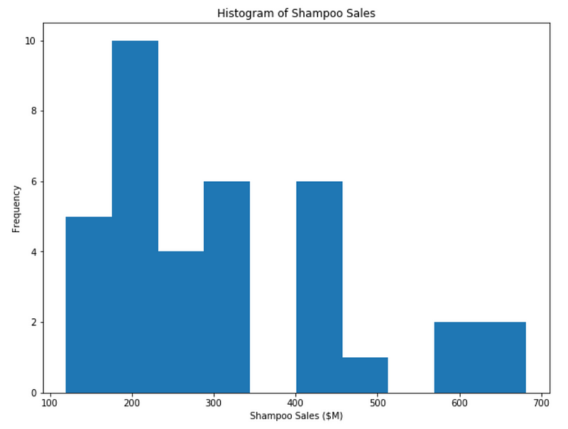
The histogram above is much better. There are numerous parameters you can change to customize the visualization to your need. For example, you can change the color and the number of bins in your histogram.

plt.figure(figsize=[10, 7.5]); # Set dimensions for figure

plt.hist(data['Sales'], bins=20, color='#fcba03')
plt.title('Histogram of Shampoo Sales');
plt.xlabel('Shampoo Sales ($M)');
plt.ylabel('Frequency');

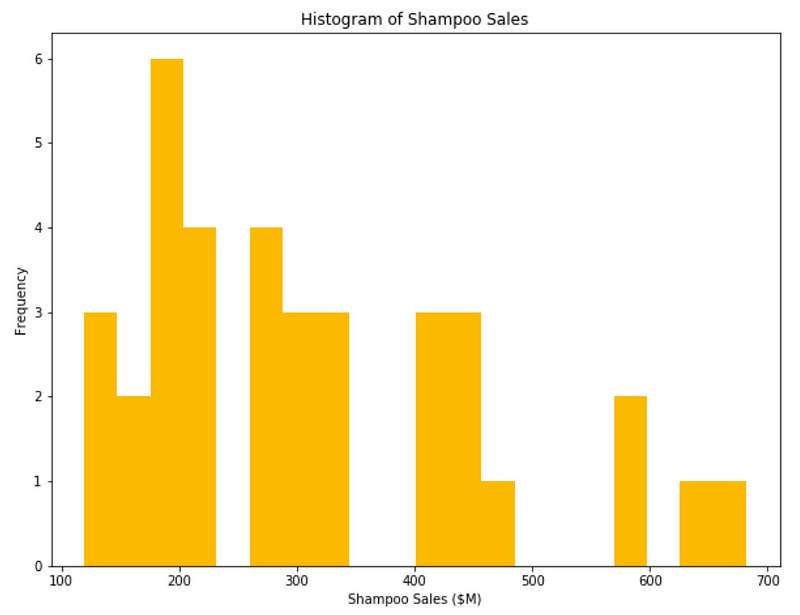
You should now be very comfortable with plotting a histogram and customizing it to your needs.

Last but not least is knowing how to display a scatter plot. Very simply, we can visualize our dataset like so:

plt.figure(figsize=[20, 7.5]); # Set dimensions for figure

sns.scatterplot(x=data['Month'], y=data['Sales']);
plt.title('Historical Shampoo Sales');
plt.ylabel('Shampoo Sales ($M)');
plt.xlabel('Month');

If you wish to learn more about plotting with the libraries we used and see how different parameters can change the plots, make sure to consult the documentation of matplotlib or seaborn.

Inferential Statistics

As the name implies, inferential statistics is the use of analysis to infer properties from a dataset.

Usually, we are looking to find a trend in our dataset that will allow us to make predictions. This is also the occasion for us to test different hypotheses.

For introductory purposes, we will use a simple linear regression to illustrate and explain inferential statistics in the context of time series.

Linear regression for time series

For this section, we will another dataset that retraces the historical concentration of CO2 in the atmosphere. Since the dataset spans 2014 years of history, let’s just consider data from 1950 and onward.

Let’s also apply what we learned before and display a scatter plot of our data.

# Dataset from here: https://www.co2.earth/historical-co2-datasets
co2_dataset = pd.read_csv('co2_dataset.csv')

plt.figure(figsize=[20, 7.5]); # Set dimensions for figure

# Let's only consider the data from the year 1950
X = co2_dataset['year'].values[1950:]
y = co2_dataset['data_mean_global'].values[1950:]

sns.scatterplot(x=X, y=y);
plt.title('Historical Global CO2 Concentration in the Atmosphere');
plt.ylabel('CO2 Concentration (ppm)');
plt.xlabel('Year');

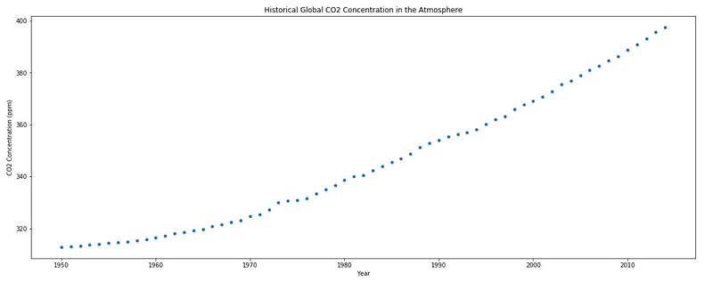
As you can see, it seems that the concentration is increasing over time.

Although the trend does not seem to be linear, it can probably still explain part of the variability of the data. Therefore, let’s make the following assumption:

• The CO2 concentration depends on time in a linear way, with some errors

Mathematically, this is expressed as:

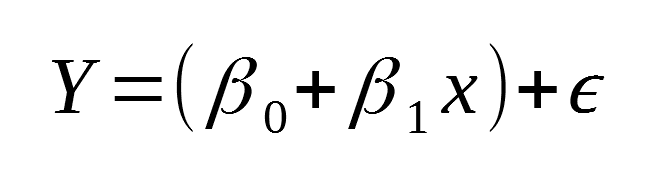
And you should easily recognize this as a linear equation with a constant term, a slope, and an error term.

It is important to note that when doing a simple linear regression, the following assumptions are made:

• the errors are normally distributed, and on average 0
• the errors have the same variance (homoscedastic)
• the errors are unrelated to each other

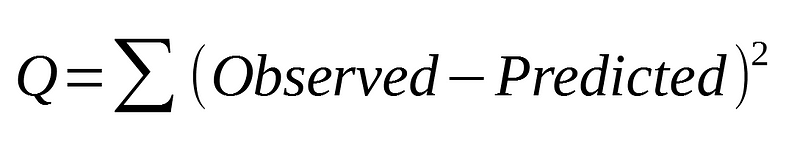
However, none of these assumptions are technically used when performing a simple linear regression. We are not generating normal distributions of the error term to estimate the parameters of our linear equation.

Instead, the ordinary least squares (OLS) is used to estimate the parameters. This is simply trying to find the minimum value of the sum of the squared error:

Linear regression in action

Let’s now fit a linear model to our data and see the estimated parameters for our model:

X = co2_dataset['year'].values[1950:].reshape(-1, 1)
y = co2_dataset['data_mean_global'].values[1950:].reshape(-1, 1)

reg = LinearRegression()

reg.fit(X, y)

print(f"The slope is {reg.coef_[0][0]} and the intercept is {reg.intercept_[0]}")

predictions = reg.predict(X.reshape(-1, 1))

plt.figure(figsize=(20, 8))
plt.scatter(X, y,c='black')
plt.plot(X, predictions, c='blue', linewidth=2)
plt.title('Historical Global CO2 Concentration in the Atmosphere');
plt.ylabel('CO2 Concentration (ppm)');
plt.xlabel('Year');
plt.show()

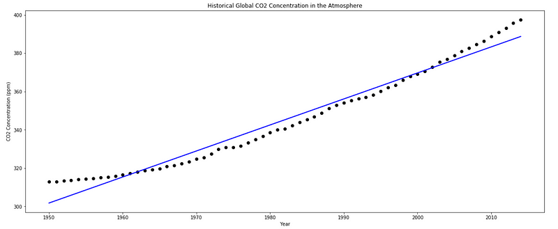
Running the piece of code above, you should the same plot and you see that the slope is 1.3589 and the intercept is -2348.

Do the parameters make sense?

The slope is indeed positive, which is normal since concentration is undoubtedly increasing.

However, the intercept is negative. Does that mean that a time 0, the concentration of CO2 is negative?

No. Our model is definitely not robust enough to go back 1950 years in time. But these parameters are the ones that minimize the sum of squared errors, hence producing the best linear fit.

Assessing the quality of the model

From the graph, we can visually say the a straight line is not the best fit to our data, but it is not the worst either.

Recall the assumption of a linear model that the errors are normally distributed. We can check this assumption by plotting a QQ-plot of the residuals.

A QQ-plot is a scatter plot of quantiles from two different distributions. If the distributions are the same, then we should see a straight line.

Therefore, if we plot a QQ-plot of our residuals against a normal distribution, we can see if they fall on a straight line; meaning that our residuals are indeed normally distributed.

X = sm.add_constant(co2_dataset['year'].values[1950:])
model = sm.OLS(co2_dataset['data_mean_global'].values[1950:], X).fit()
residuals = model.resid
qq_plot = sm.qqplot(residuals, line='q')
plt.show()

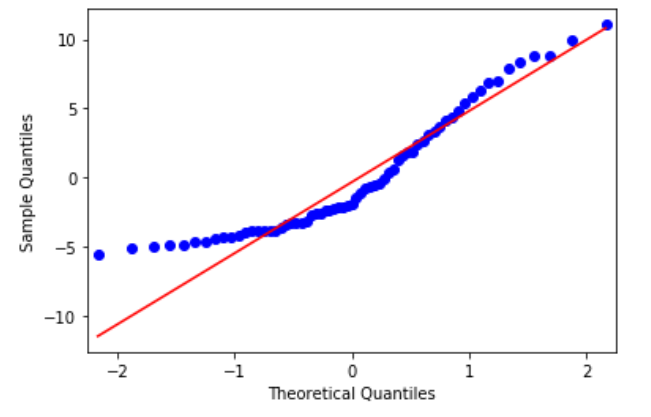
As you can see, the blue dots represent the residuals, and they do not fall on a straight line. Therefore, they are not normally distributed, and this is an indicator that a linear model is not the best fit to our data.

This can be further supported by plotting a histogram of the residuals:

X = sm.add_constant(co2_dataset['year'].values[1950:])
model = sm.OLS(co2_dataset['data_mean_global'].values[1950:], X).fit()
residuals = model.resid

plt.hist(residuals);

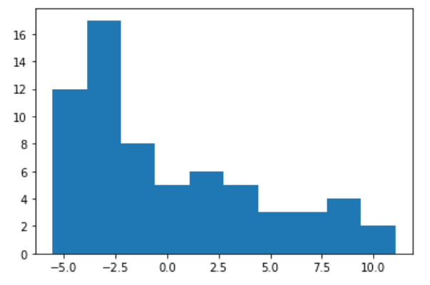
Again, we can clearly see that it is not a normal distribution.

Hypothesis testing

A major component of inferential statistics is hypothesis testing. This is a way to determine if the observed trend is due to randomness, or if there is a real statistical significance.

For hypothesis testing, we must define a hypothesis and a null hypothesis. The hypothesis is usually the trend we are trying to extract from data, while the null hypothesis is its exact opposite.

Let’s define the hypotheses for our case:

• hypothesis: there is a linear correlation between time and CO2 concentration
• null hypothesis: there is no linear correlation between time and CO2 concentration

Awesome! Now, let’s fit a linear model to our dataset using another library that will automatically run hypothesis tests for us:

X = sm.add_constant(co2_dataset['year'].values[1950:])
model = sm.OLS(co2_dataset['data_mean_global'].values[1950:], X).fit()
print(model.summary())

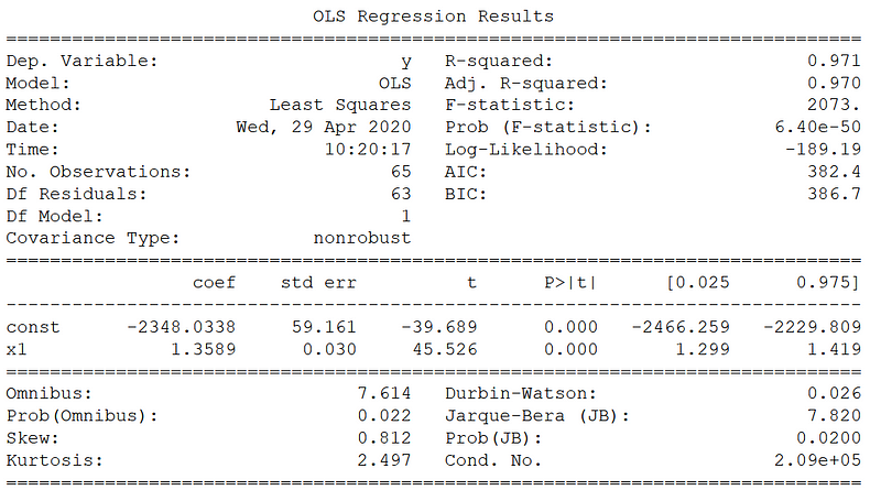
Now, there is a lot of information here, but let’s consider only a few numbers.

First, we have a very high R² value of 0.971. This means that more than 97% of the variability in CO2 concentration is explained with the time variable.

Then, the F-statistic is very large as well: 2073. This means that there is statistical significance that a linear correlation exists between time and CO2 concentration.

Finally, looking at the p-value of the slope coefficient, you notice that it is 0. While the number is probably not 0, but still very small, it is another indicator of statistical significance that a linear correlation exists.

Usually, a threshold of 0.05 is used for the p-value. If less, the null hypothesis is rejected.

Therefore, because of a large F-statistic, in combination with a small p-value, we can reject the null hypothesis.

That’s it! You are now in a very good position to kick start your time series analysis project!

With these basic concepts, we will build upon them to make better models to help us forecast time series data.

Make sure to grab my free time series cheat sheet for future reference!

Cheers!

Support me

Enjoying my work? Show your support with Buy me a coffee, a simple way for you to encourage me, and I get to enjoy a cup of coffee! If you feel like it, just click the button below 👇