Advanced Time Series Analysis with ARMA and ARIMA

Introduction

In previous articles, we introduced moving average processes MA(q), and autoregressive processes AR(p) as two ways to model time series. Now, we will combine both methods and explore how ARMA(p,q) and ARIMA(p,d,q) models can help us to model and forecast more complex time series.

This article will cover the following topics:

• ARMA models
• ARIMA models
• Ljung-Box test
• Akaike information criterion (AIC)

By the end of this article, you should be comfortable with implementing ARMA and ARIMA models in Python and you will have a checklist of steps to take when modelling time series.

The notebook and dataset are here.

Let’s get started!

Get the latest forecasting techniques, covering both statistical and deep learning models in Python, with my free time series cheat sheet!

ARMA Model

Recall that an autoregressive process of order p is defined as:

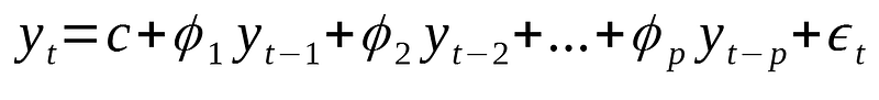
Where:

• p is the order
• c is a constant
• epsilon: noise

Recall also that a moving average process q is defined as:

Where:

• q is the order
• c is a constant
• epsilon is noise

Then, an ARMA(p,q) is simply the combination of both models into a single equation:

Hence, this model can explain the relationship of a time series with both random noise (moving average part) and itself at a previous step (autoregressive part).

Let’s how an ARMA(p,q) process behaves with a few simulations.

Simulate and ARMA(1,1) process

Let’s start with a simple example of an ARMA process of order 1 in both its moving average and autoregressive part.

First, let’s import all libraries that will be required throughout this tutorial:

from statsmodels.graphics.tsaplots import plot_pacf
from statsmodels.graphics.tsaplots import plot_acf
from statsmodels.tsa.arima_process import ArmaProcess
from statsmodels.stats.diagnostic import acorr_ljungbox
from statsmodels.tsa.statespace.sarimax import SARIMAX
from statsmodels.tsa.stattools import adfuller
from statsmodels.tsa.stattools import pacf
from statsmodels.tsa.stattools import acf
from tqdm import tqdm_notebook
import matplotlib.pyplot as plt
import numpy as np
import pandas as pd

import warnings
warnings.filterwarnings('ignore')

%matplotlib inline

Then, we will simulate the following ARMA process:

In code:

ar1 = np.array([1, 0.33])
ma1 = np.array([1, 0.9])

simulated_ARMA_data = ArmaProcess(ar1, ma1).generate_sample(nsample=10000)

We can now plot the first 200 points to visualize our generated time series:

plt.figure(figsize=[15, 7.5]); # Set dimensions for figure
plt.plot(simulated_ARMA_data)
plt.title("Simulated ARMA(1,1) Process")
plt.xlim([0, 200])
plt.show()

And you should get something similar to:

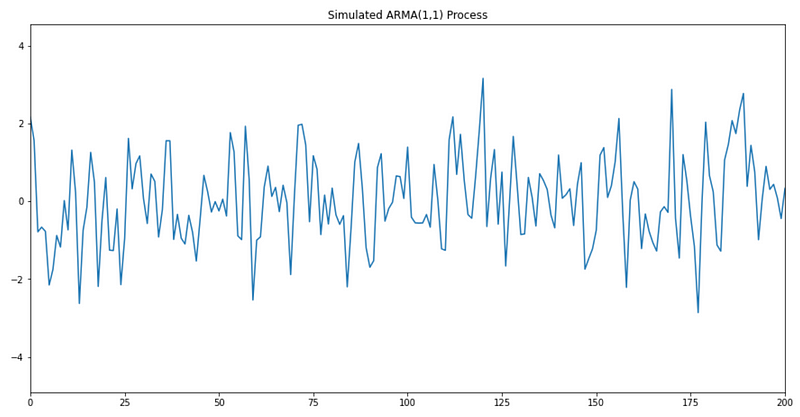
Then, we can take a look at the ACF and PACF plots:

plot_pacf(simulated_ARMA_data);
plot_acf(simulated_ARMA_data);

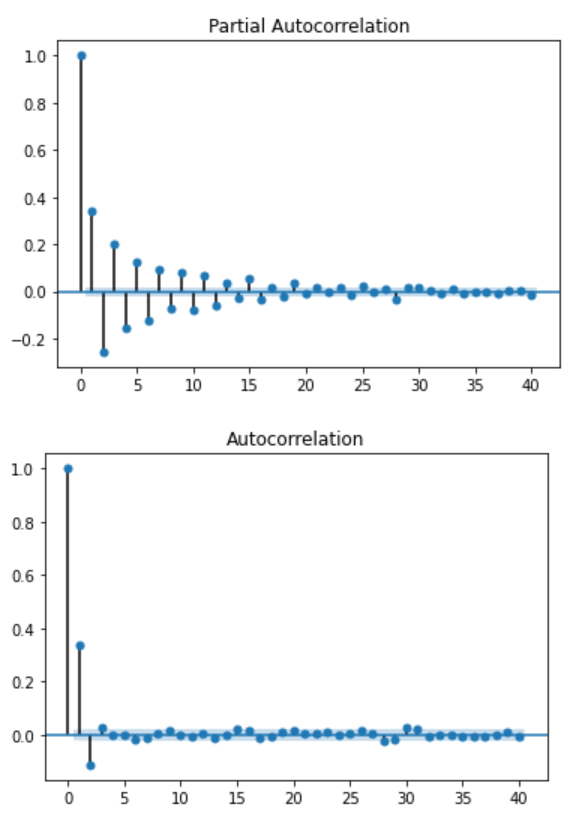
As you can see, we cannot infer the order of the ARMA process by looking at these plots. In fact, looking closely, we can see some sinusoidal shape in both ACF and PACF functions. This suggests that both processes are in play.

Simulate an ARMA(2,2) process

Similarly, we can simulate an ARMA(2,2) process. In this example, we will simulate the following equation:

In code:

ar2 = np.array([1, 0.33, 0.5])
ma2 = np.array([1, 0.9, 0.3])

simulated_ARMA2_data = ArmaProcess(ar1, ma1).generate_sample(nsample=10000)

Then, we can visualize the simulated data:

plt.figure(figsize=[15, 7.5]); # Set dimensions for figure
plt.plot(simulated_ARMA2_data)
plt.title("Simulated ARMA(2,2) Process")
plt.xlim([0, 200])
plt.show()

Looking at the ACF and PACF plots:

plot_pacf(simulated_ARMA2_data);
plot_acf(simulated_ARMA2_data);

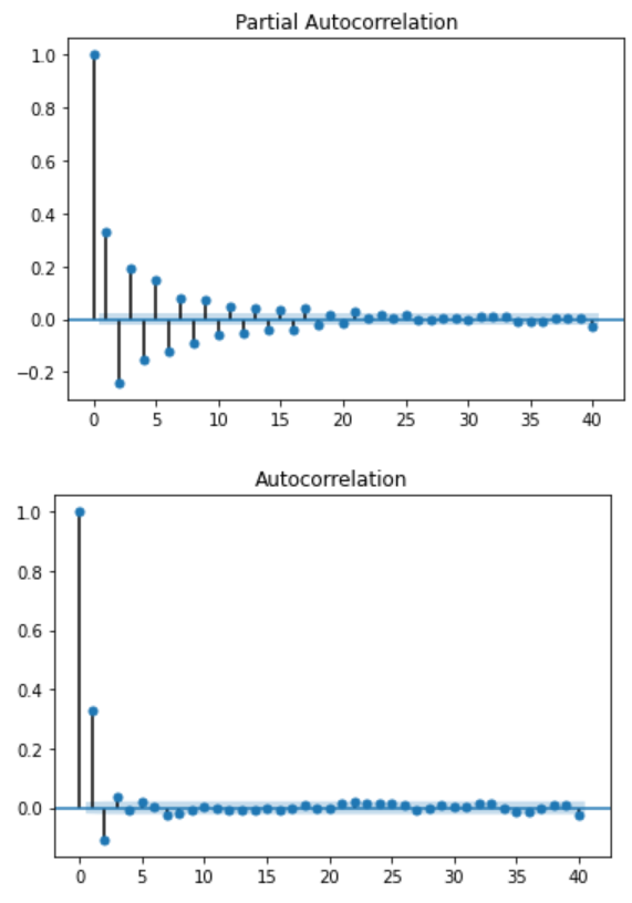
As you can see, both plots exhibit the same sinusoidal trend, which further supports the fact that both an AR(p) process and a MA(q) process is in play.

ARIMA Model

ARIMA stands for AutoRegressive Integrated Moving Average.

This model is the combination of autoregression, a moving average model and differencing. In this context, integration is the opposite of differencing.

Differencing is useful to remove the trend in a time series and make it stationary.

It simply involves subtracting a point a t-1 from time t. Realize that you will, therefore, lose the first data point in a time series if you apply differencing once.

Mathematically, the ARIMA(p,d,q) now requires three parameters:

• p: the order of the autoregressive process
• d: the degree of differencing (number of times it was differenced)
• q: the order of the moving average process

and the equations is expressed as:

Just like with ARMA models, the ACF and PACF cannot be used to identify reliable values for p and q.

However, in the presence of an ARIMA(p,d,0) process:

• the ACF is exponentially decaying or sinusoidal
• the PACF has a significant spike at lag p but none after

Similarly, in the presence of an ARIMA(0,d,q) process:

• the PACF is exponentially decaying or sinusoidal
• the ACF has a significant spike at lag q but none after

Let’s walk through an example of modelling with ARIMA to get some hands-on experience and better understand some modelling concepts.

Project —Modelling the quarterly EPS for Johnson&Johnson

Let’s revisit a dataset that we analyzed previously. This dataset was used to show the Yule-Walker equation can help us estimate the coefficients of an AR(p) process.

Now, we will use the same dataset, but model the time series with an ARIMA(p,d,q) model.

You can grab the notebook or download the dataset to follow along.

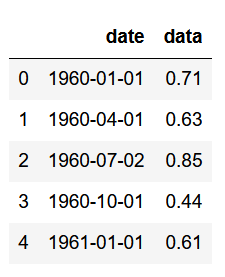
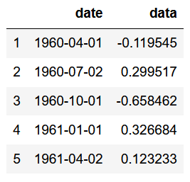
First, we import the dataset and display the first five rows:

data = pd.read_csv('jj.csv')
data.head()

Then, let’s plot the entire dataset:

plt.figure(figsize=[15, 7.5]); # Set dimensions for figure
plt.scatter(data['date'], data['data'])
plt.title('Quarterly EPS for Johnson & Johnson')
plt.ylabel('EPS per share ($)')
plt.xlabel('Date')
plt.xticks(rotation=90)
plt.grid(True)
plt.show()

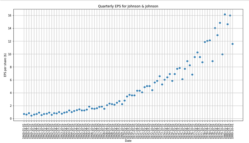
As you can see, there is both a trend and a change in variance in this time series.

Let’s plot the ACF and PACF functions:

plot_pacf(data['data']);
plot_acf(data['data']);

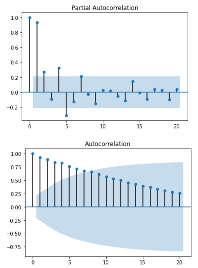
As you can see, there is no way of determining the right order for the AR(p) process or MA(q) process.

The plots above are also a clear indication of non-stationarity. To further prove this point, let’s use the augmented Dicker-Fuller test:

# Augmented Dickey-Fuller test

ad_fuller_result = adfuller(data['data'])
print(f'ADF Statistic: {ad_fuller_result[0]}')
print(f'p-value: {ad_fuller_result[1]}')

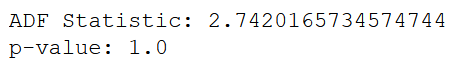
Here, the p-value is larger than 0.05, meaning the we cannot reject the null hypothesis stating that the time series is non-stationary.

Therefore, we must apply some transformation and some differencing to remove the trend and remove the change in variance.

We will hence take the log difference of the time series. This is equivalent to taking the logarithm of the EPS, and then apply differencing once. Note that because we are differencing once, we will get rid of the first data point.

# Take the log difference to make data stationary

data['data'] = np.log(data['data'])
data['data'] = data['data'].diff()
data = data.drop(data.index[0])
data.head()

Now, let’s plot the new transformed data:

plt.figure(figsize=[15, 7.5]); # Set dimensions for figure
plt.plot(data['data'])
plt.title("Log Difference of Quarterly EPS for Johnson & Johnson")
plt.show()

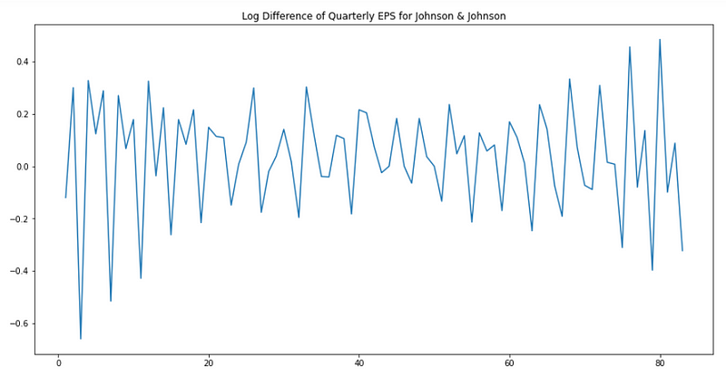
It seems that trend and the change in variance were removed, but we want to make sure that it is the case. Therefore, we apply the augmented Dickey-Fuller test again to test for stationarity.

# Augmented Dickey-Fuller test

ad_fuller_result = adfuller(data['data'])
print(f'ADF Statistic: {ad_fuller_result[0]}')
print(f'p-value: {ad_fuller_result[1]}')

This time, the p-value is less than 0.05, we reject the null hypothesis, and assume that the time series is stationary.

Now, let’s look at the PACF and ACF to see if we can estimate the order of one of the processes in play.

plot_pacf(data['data']);
plot_acf(data['data']);

Examining the PACF above, it seems that there is an AR process of order 3 or 4 in play. However, the ACF is not informative and we see some sinusoidal shape.

Therefore, how can we make sure that we choose the right order for both the AR(p) and MA(q) processes?

We will need try different combinations of orders, fit an ARIMA model with those orders, and use a criterion for order selection.

This brings us to the topic of Akaike’s Information Criterion or AIC.

Akaike’s Information Criterion (AIC)

This criterion is useful for selecting the order (p,d,q) of an ARIMA model. The AIC is expressed as:

Where L is the likelihood of the data and k is the number of parameters.

In practice, we select the model with the lowest AIC compared to other models.

It is important to note that the AIC cannot be used to select the order of differencing (d). Differencing the data will the change the likelihood (L) of the data. The AIC of models with different orders of differencing are therefore not comparable.

Also, notice that since we select the model with the lowest AIC, more parameters will increase the AIC score and thus penalize the model. While a model with more parameters could perform better, the AIC is used to find the model with the least number of parameters that will still give good results.

A final note on AIC is that it can only be used relative to other models. A small AIC value is not a guarantee that the model will have a good performance on unsee data, or that its SSE will be small.

Now that we know how we will base our decision to select the best order for the ARIMA model, let’s write a function that will test all orders for us.

def optimize_ARIMA(order_list, exog):
    """
        Return dataframe with parameters and corresponding AIC
        
        order_list - list with (p, d, q) tuples
        exog - the exogenous variable
    """
    
    results = []
    
    for order in tqdm_notebook(order_list):
        try: 
            model = SARIMAX(exog, order=order).fit(disp=-1)
        except:
            continue
            
        aic = model.aic
        results.append([order, model.aic])
        
    result_df = pd.DataFrame(results)
    result_df.columns = ['(p, d, q)', 'AIC']
    #Sort in ascending order, lower AIC is better
    result_df = result_df.sort_values(by='AIC', ascending=True).reset_index(drop=True)
    
    return result_df

The function above will result in a dataframe that will list the orders and the corresponding AIC, starting with the best model on top.

We will try all combinations with orders (p,q) ranging from 0 to 8, but keeping the differencing order equal to 1.

ps = range(0, 8, 1)
d = 1
qs = range(0, 8, 1)

# Create a list with all possible combination of parameters
parameters = product(ps, qs)
parameters_list = list(parameters)

order_list = []

for each in parameters_list:
    each = list(each)
    each.insert(1, 1)
    each = tuple(each)
    order_list.append(each)
    
result_df = optimize_ARIMA(order_list, exog=data['data'])

result_df

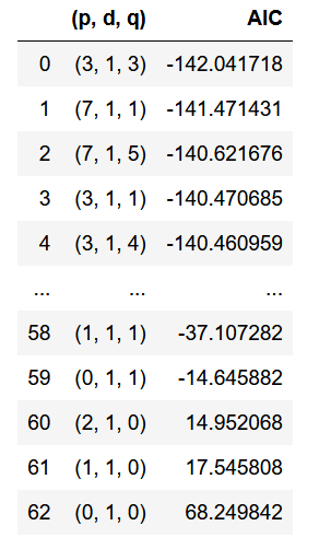
Once the function is done running, you should see that the order associated with the lowest AIC is (3,1,3). Therefore, this suggests are ARIMA model with an AR(3) process and a MA(3) process.

Now, we can print a summary of the best model, which an ARIMA (3,1,3).

best_model = SARIMAX(data['data'], order=(3,1,3)).fit()
print(best_model.summary())

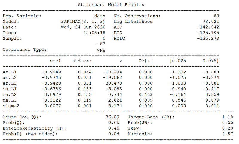
From the summary above, we can see the value for all coefficients and their associated p-values. Notice how the parameter for the MA process at lag 2 does not seem to be statistically significant according to the p-value. Still, let’s keep it in the model for now.

Hence, from the table above, the time series can be modeled as:

Where epsilon is noise with a variance of 0.0077.

The final part of modelling a time series is to study the residuals.

Ideally, the residuals will be white noise, with no autocorrelation.

A good way to test this is to use the Ljung-Box test. Note that this test can only be applied to the residuals.

# Ljung-Box test
ljung_box, p_value = acorr_ljungbox(best_model.resid)

print(f'Ljung-Box test: {ljung_box[:10]}')
print(f'p-value: {p_value[:10]}')

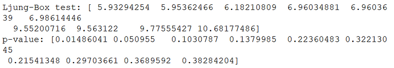
Here, the null hypothesis for the Ljung-Box test is that there is no autocorrelation. Looking at the p-values above, we can see that they are above 0.05. Therefore, we cannot reject the null hypothesis, and the residuals are indeed not correlated.

We can further support that by plotting the ACF and PACF of the residuals.

plot_pacf(best_model.resid);
plot_acf(best_model.resid);

As you can see, the plots above resemble those of white noise.

Therefore, this model is ready to be used for forecasting.

General Modelling Procedure

Here is a general procedure that you can follow whenever you are faced with a time series:

1. Plot the data and identify unsual observations. Understand the pattern of the data.
2. Apply a transormation or differencing to remove the trend and stabilize the variance
3. Test for stationarity. If the series is not stationary, apply another transformation or differencing.
4. Plot the ACF and PACF to maybe estimate the order of the MA or AR process.
5. Try different combinations of orders and select the model with the lowest AIC.
6. Check the residuals and make sure that they look like white noise. Apply the Ljung-Box test to make sure.
7. Calculate forecasts.

Conclusion

Congratulations! You now understand what an ARMA model is and you understand how to use non-seasonal ARIMA models for advanced time series analysis. You also have a road map for time series analysis that you can apply to make sure that you obtain the best model possible.

Get the latest forecasting techniques in Python with my free time series cheat sheet!

Cheers 🍺

Support me

Enjoying my work? Show your support with Buy me a coffee, a simple way for you to encourage me, and I get to enjoy a cup of coffee! If you feel like it, just click the button below 👇